A Reliable Contextual Bandit Algorithm: LinUCB
Posted: Updated:
A user visits a news website. Which articles should they be shown?
This question was the target of the paper A Contextual-Bandit Approach to Personalized News Article Recommendation, which introduced the now famous LinUCB contextual bandit algorithm. In fact, personalizing news is just one application. Others include:
- Dynamic Pricing: Which discounts should be offered to maximize profit?
- Personalized Advertising: Which advertisements should be shown to maximize clicks?
- Medical Trials: Which treatments should be prescribed to maximize survival?
To see how it applies generally, it helps to understand the personalized news application in more detail. When a user arrives at a website, they are represented as a feature vector. This may measure their gender, geography, age, device, or anything else considered relevant. Also, each recommendable article is represented with a feature vector. This may measure the article’s topic, category, geography and date. Together, the user’s and articles’ features are considered the ‘context’ of the recommendation. LinUCB is an algorithm that, when given a context, will select an article the user is likely to click.
However, the articles need not be actual articles. It is any set of actions where each is represented as a vector. A user need not be an actual user. It is any single vector describing the circumstance of the decision. The goal need not be click-through-rate, but rather any value dependent on the context and action selected. Within this framework, linUCB can be applied to dynamic pricing, advertising, medical trials and others.
This Post
In this post, I’ll explain the LinUCB algorithm from the ground up. I selected it for its utility. It is broadly applicable and strikes an attractive balance of simplicity and flexibility, making it a reliable choice for real world problems.
Since I’d like to communicate intuition, I will only focus on the disjoint variant. This is ‘Algorithm 1’ from the paper. The difference with ‘Algorithm 2’ is the disjoint variant omits shared features, features that are the same across actions. The user features described earlier are shared features. The article features are non-shared features. In practice, shared features are essential and in fact, more common than non-shared features. However, they are not essential for understanding the algorithm. Algorithm 2 is the same idea, slightly expanded.
To begin, I’ll state the problem generally and a bit redundantly.
Stochastic Contextual Bandits with Linear Payoffs
The contextual bandit problem is as follows. In each of \(T\) rounds, we select one of several actions, each represented with a vector. For the action selected, we observe and obtain a reward whose expectation is a linear function of the selected vector. The reward then becomes part of data to inform future selections. The goal is to maximize cumulative reward over all rounds.
To introduce notation and restate this precisely, round \(t = 1, 2, \cdots, T\) proceeds in steps:
For each of \(K_t\) actions, a vector is observed: \(\{\mathbf{x}_{t, k} \mid k = 1, 2, \cdots, K_t\}\)1. This is the context of the decision. Note there are no shared features.
Based on the vectors and their relationships with rewards learned from previous observations, an algorithm \(\mathsf{A}\) selects an action \(a_t \in \{1, \cdots, K_t\}\).
A reward \(r_{t, a_t}\) is observed, sampled independently from an unknown distribution dependent on the context and action selected. This makes the problem stochastic. To be explicit, the unchosen rewards \(r_{t, k}\) where \(k \neq a_t\) are unobserved.
The reward expectation is linearly related to the context, making the problem with linear payoffs:
\[\mathbb{E}\big[r_{t, k} \vert \mathbf{x}_{t, k} \big] = \mathbf{x}_{t, k}^{\top}\boldsymbol{\theta}_{k}\]where \(\{\boldsymbol{\theta}_k \mid k = 1, 2, \cdots, K_t\}\) are unknown ‘true’ parameters. Also, the unknown reward distribution is bounded. A common bound is \([0, 1]\).
The goal is to design an \(\mathsf{A}\) that maximizes the sum of rewards over rounds. As data rolls in, \(\mathsf{A}\) learns a policy \(\pi\), which maps features to a selected action. A performant algorithm will, in minimal rounds, learn enough about the \(\boldsymbol{\theta}_k\)’s to develop a high reward \(\pi\).
To ground this, we’ll start with a simple example where the true parameters, the \(\boldsymbol{\theta}_k\)’s, are known.
Known Parameters
We suppose in all rounds, there are only two actions, represented with a single number (not counting an intercept term) and the parameters are known. Prior to selecting an action, this can be represented as:
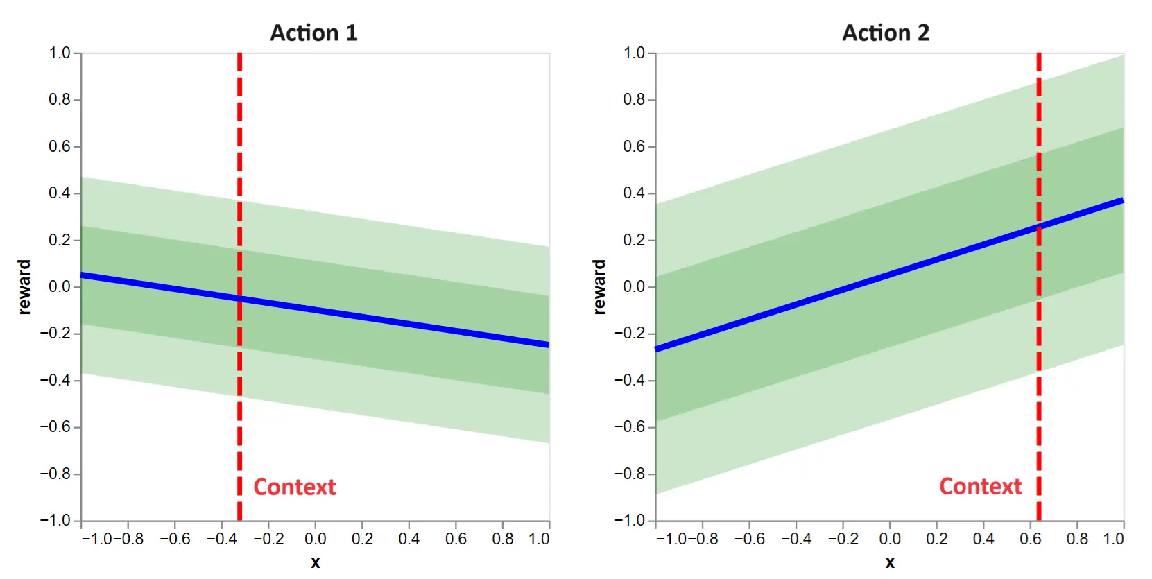 Figure 1: This shows the contextual bandit decision to make when action functions are known. The blue lines tells us \(\mathbb{E}[r_{0, k}|x]\), the expected reward as a function of the context for the actions \(k=1\) and \(k=2\). The vertical lines give us the contexts for the first round: \(x_{0, 1}\) and \(x_{0, 2}\). The green bands give us standard deviations of \(r_{0, k}\) around its expected value.
The contexts are shown with vertical lines. Since \(\boldsymbol{\theta}_1\) and \(\boldsymbol{\theta}_2\) are known, we can see the linear relationship between contexts and expected rewards. We refer to these as action functions. Further, one and two standard deviation bands are shown, highlighting the reward distributions.
Recalling the goal to maximize reward, which action would you select? That is, in figure 1, would you select action 1 on the left or action 2 on the right?
Clearly, we should choose action 2, because it yields a higher expected reward, indicated with the horizontal lines.
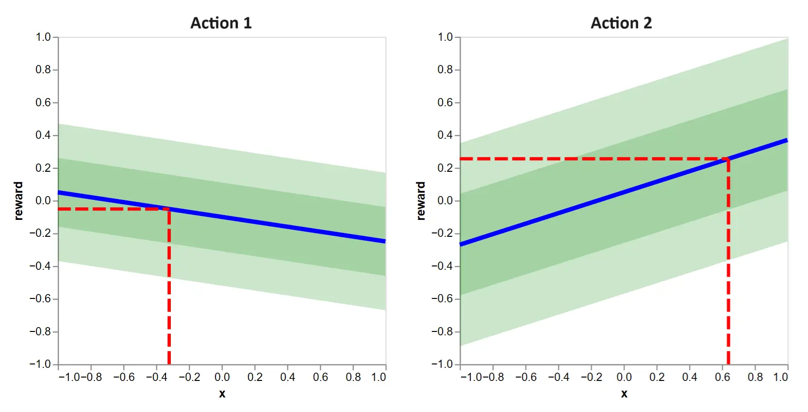 Figure 2: This tells us the decision criteria when action functions are known. Simply pick the action which yields the higher expected reward given the context. In this case, it is action 2.
Following the selection, we observe a reward of only the selected action. Due to noise, it is not equal to the expected reward. Selecting \(a_1 = 2\) gives us our first observed data point:
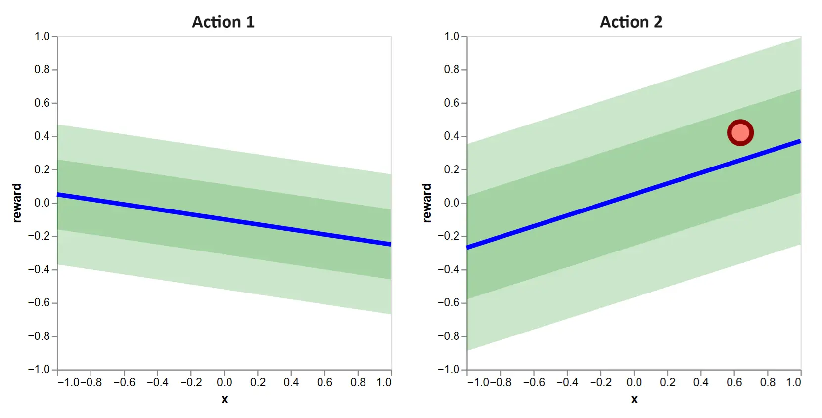 Figure 3: After making a selection, we observe a sampled reward, indicated as a dot at the chosen context.
All of this is to illustrate the information available prior to a decision, the decision itself and the information gained with a decision. It is crucial to crystalize this repeating process when working with contextual bandits.
Lastly, because the action functions are known, we can determine the optimal policy \(\pi^*\) and its expected reward by taking the max across action functions:
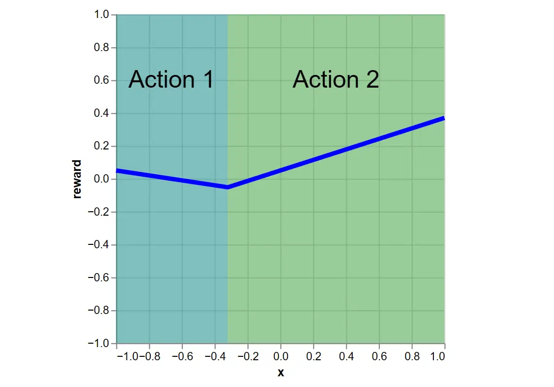 Figure 4: This is the optimal policy. It chooses the max expected reward action for any \(x\). The blue line is the policy’s expected reward.
Unknown Parameters
Knowing the true parameters makes the above a trivial case. The complexity arises when the parameters2 are unknown. In this case, selecting an action has two purposes:
- Obtain a high reward.
- Obtain information needed to make future high reward selections.
This is the fundamental challenge of bandits, known as the exploration-exploitation trade-off.
To see it, let’s play the same game, but with unknown action functions. The first round begins with the context:
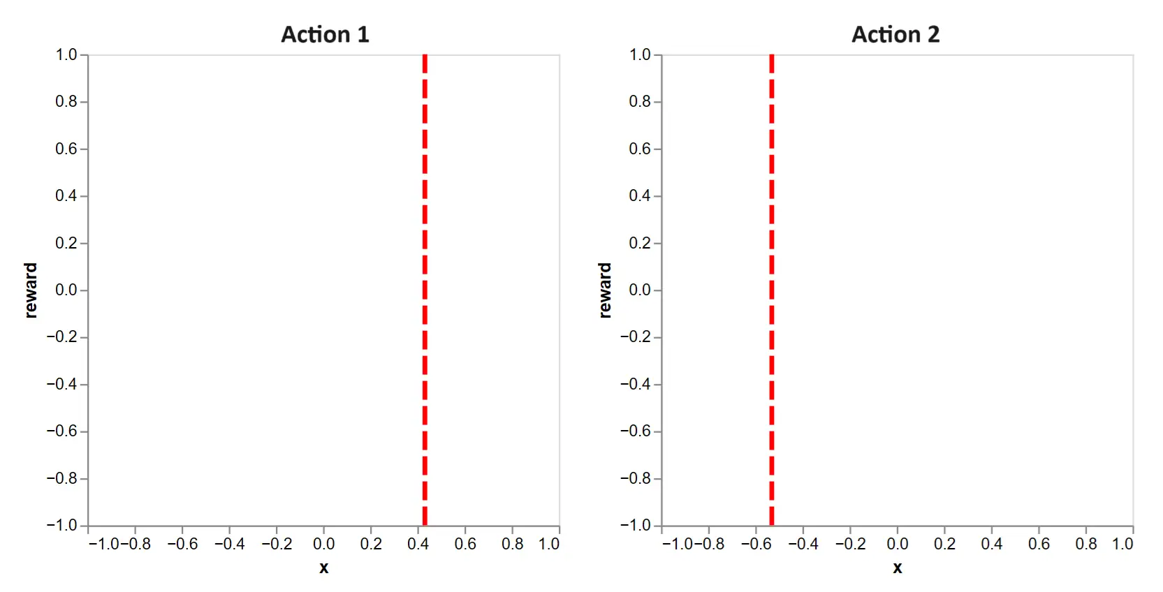 Figure 5: With unknown action functions, we face the following decision in round 1. Clearly, there is no information to favor one action over the other.
A Naive Approach
In round \(t=1\), we have no data, so we may as well guess randomly. In fact, the second round will be subject to the same, albeit slightly ameliorated, problem and so, the next round might as well be random as well. This suggests a naive algorithm:
-
Randomly select an action for the first 100 rounds.
-
Fit a linear regression model for each action.
-
For all future rounds, use the fitted linear models as though they were the true action functions.
Let’s call this the ‘explore-then-exploit’ approach. After 100 exploratory rounds, we have data and a fit like this:
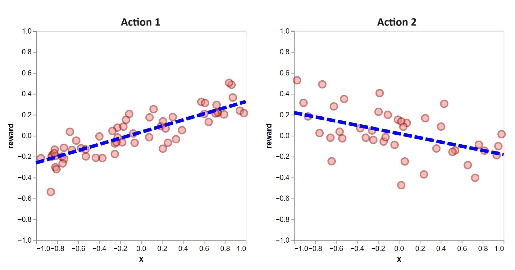 Figure 6: The dotted lines are the estimated action functions after 100 exploratory rounds of randomly selected actions.
Going forward, we select the action which, given the context, yields a higher value.
The question is: how will it perform?
To answer that, we need to discuss the contextual bandit community’s favor metric, regret. To get there, we start with something simpler.
Expected Payoff
A natural metric of the learning algorithm \(\mathsf{A}\) is the total \(T\)-round payoff:
\[\sum_{t=1}^T r_{t, a_t}\]This, however, is a random variable. Running \(\mathsf{A}\) through a contextual bandits simulation twice will give two different values. So some of it speaks to the randomness of the simulation. We prefer the expected payoff:
\[\mathbb{E}\Big[\sum_{t=1}^T r_{t, a_t}\Big]\]If we run \(\mathsf{A}\) for \(S\) simulations of \(T\)-rounds, this value is what the average payoff approaches as \(S \rightarrow \infty\). It is a more pure evaluation of \(\mathsf{A}\) than the payoff. Note that in addition to \(\mathsf{A}\), it depends on \(T\) and the environment.
However, the expected payoff lacks something important. To see this, we plot it as a function of \(T\) for the explore-then-exploit algorithm:
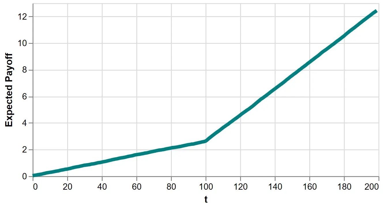 Figure 7: Expected payoff of the 100-round explore-then-exploit algorithm.
Is this good? It’s increasing, but how much is good enough? Notice it’s increasing for the first 100 rounds where we select actions randomly. This is because rewards for both actions are, on average, slightly positive. So increasing payoff is no indication of a performant algorithm.
The problem is there’s no benchmark.
Regret
Regret measures performance against the optimal policy, the policy derived knowing the true action functions. It’s the policy we derived in the trivial game played in the ‘Known Parameters’ section. Following the definition3 in Li (2010), it’s written as:
\[R_\mathsf{A}(T) = \underbrace{\mathbb{E}\Big[\sum_{t=1}^T r_{t, a_t^*}\Big]}_{\substack{\textrm{Expected payoff} \\ \textrm{of optimal policy}}} - \underbrace{\mathbb{E}\Big[\sum_{t=1}^T r_{t, a_t}\Big]}_{\substack{\textrm{Expected payoff} \\ \textrm{of }\mathsf{A}}}\]This is better. If and when \(R_\mathsf{A}(T)\) flattens out, the additional rounds create near-zero terms, meaning \(\mathsf{A}\) has learned approximately the optimal policy.
Let’s view it for the explore-then-exploit algorithm:
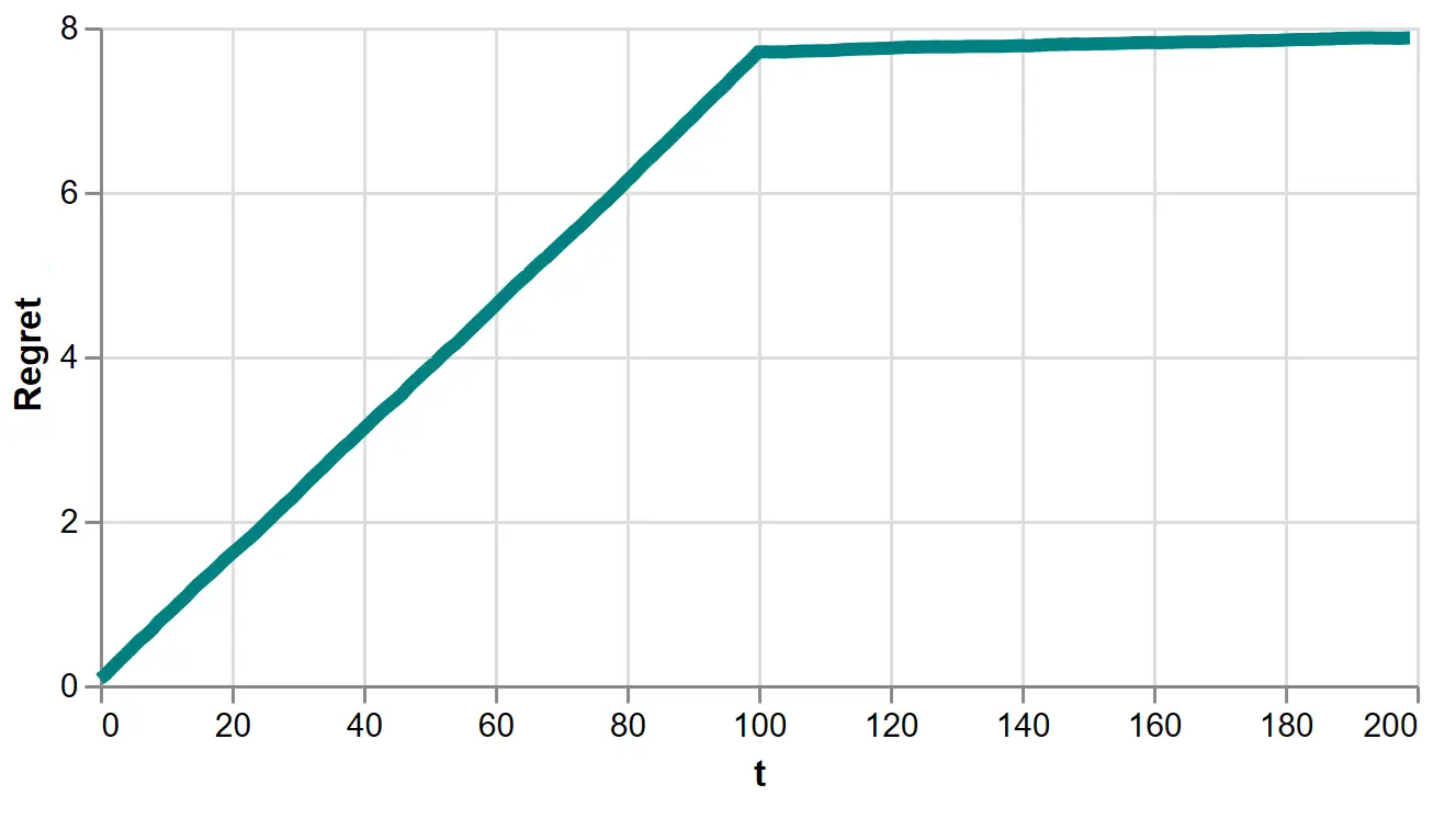 Figure 7: Regret of the 100-round explore-then-exploit algorithm
This is more informative. We see each exploratory round accrues a constant increment of regret, creating an upward sloping line. On the 101-th round, we approximately learn the optimal policy, so the increments of regret fall to near zero, creating a near flat line.
The kink at \(t=100\) suggests regret strongly depends on the number of exploratory rounds, so we vary that value next:
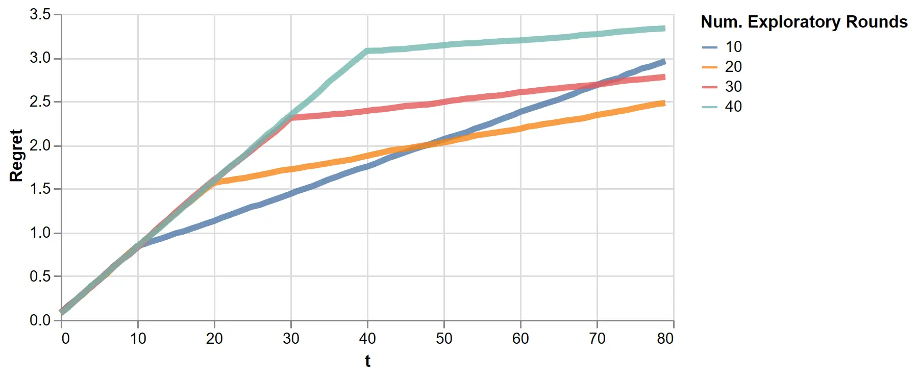 Figure 9: The regret of the exploit-then-exploit algorithm with varying exploratory rounds
This clearly shows the explore-exploit trade-off. With a few exploratory rounds, we reduce the length of the initial steep incline but pay for it with a positive slope in the exploit rounds. With more exploration, this long term slope is reduced.
One might tune the number of exploratory rounds, but doing so requires knowing the total number of rounds \(T\) upfront, which is only sometimes true in practice. Fortunately, LinUCB offers a better solution.
Before we get into it, I’ll make a few general comments on regret.
-
Computing regret requires the optimal policy. In applications, the optimal policy is unknown, so regret is unknown. It is only known in theoretical or simulated environments. It is assumed, without controversy, an \(\mathsf{A}\) with performant regret in such environments will perform well in the real world.
-
Regret, as defined here as a difference of expectations, is always non-decreasing in \(T\). This is because in every round, no learning algorithm, after observing finite data, can produce a policy better than the optimal policy in expectation. Therefore, the goal is for \(R_\mathsf{A}(T)\) to grow as slowly as possible.
-
Outside of plots, an algorithm’s regret is expressed as a category of increasing function of \(T\) and often of other variables, like the dimensionality of the context \(d\) or the number of actions \(K\). For instance, an algorithm might achieve ‘\(O(d\sqrt{TK})\) regret,’ meaning it eventually always remains less than \(cd\sqrt{TK}\) for some constant \(c\). See Table 2 of Zhou (2016) for a list of algorithms and their regret, albeit sometimes defined differently than here.
-
Revealing my applied-consultant-non-academic side, I believe regret receives extra attention in the literature because bounds on it can be proven, unlike most reinforcement learning metrics. Indeed, often an algorithm is sold on a proof of an attractively slow growing regret bound.
However in my experience, regret is not sufficient for selecting the best algorithm for an application. Regret is conditional on an idealized environment, which may only approximate the real world. In Bietti (2021), after evaluating several algorithms against a large number of supervised learning datasets, the authors discovered performance often ran counter to what the theory suggests.
Also, compute efficiency matters. An algorithm that is slow to run may be impossible to improve iteratively.
Lastly, simple, easy-to-debug algorithms are preferred, since evaluation and getting targeted feedback in live environments is challenging.
LinUCB: the Idea
With the problem defined, we move onto the LinUCB algorithm, the ‘disjoint’ variate described in Li (2010). “Lin” refers to the linearity assumption relating contexts to expected rewards. “UCB” refers to a broad class of upper confidence bound algorithms, which establish a simple approach to the exploration-exploitation trade-off. For every action, they estimate a confidence interval around its expected reward and select the action with the highest upper confidence bound. This is referred to as an ‘optimism under uncertainty’ heuristic, and empirically, it performs well.
Further, the linearity assumption and optimism heuristic work quite nicely together. The upper bound can be computed analytically and updated in each round. As we’ll see, the algorithm essentially runs \(K\) online ridge regressions, which bring convenient Bayesian computations of confidence4 intervals.
To motivate this, suppose the explore-then-exploit approach applied ridge regression following the initial 100 exploratory rounds. On the next round, we face the contexts of the vertical lines:
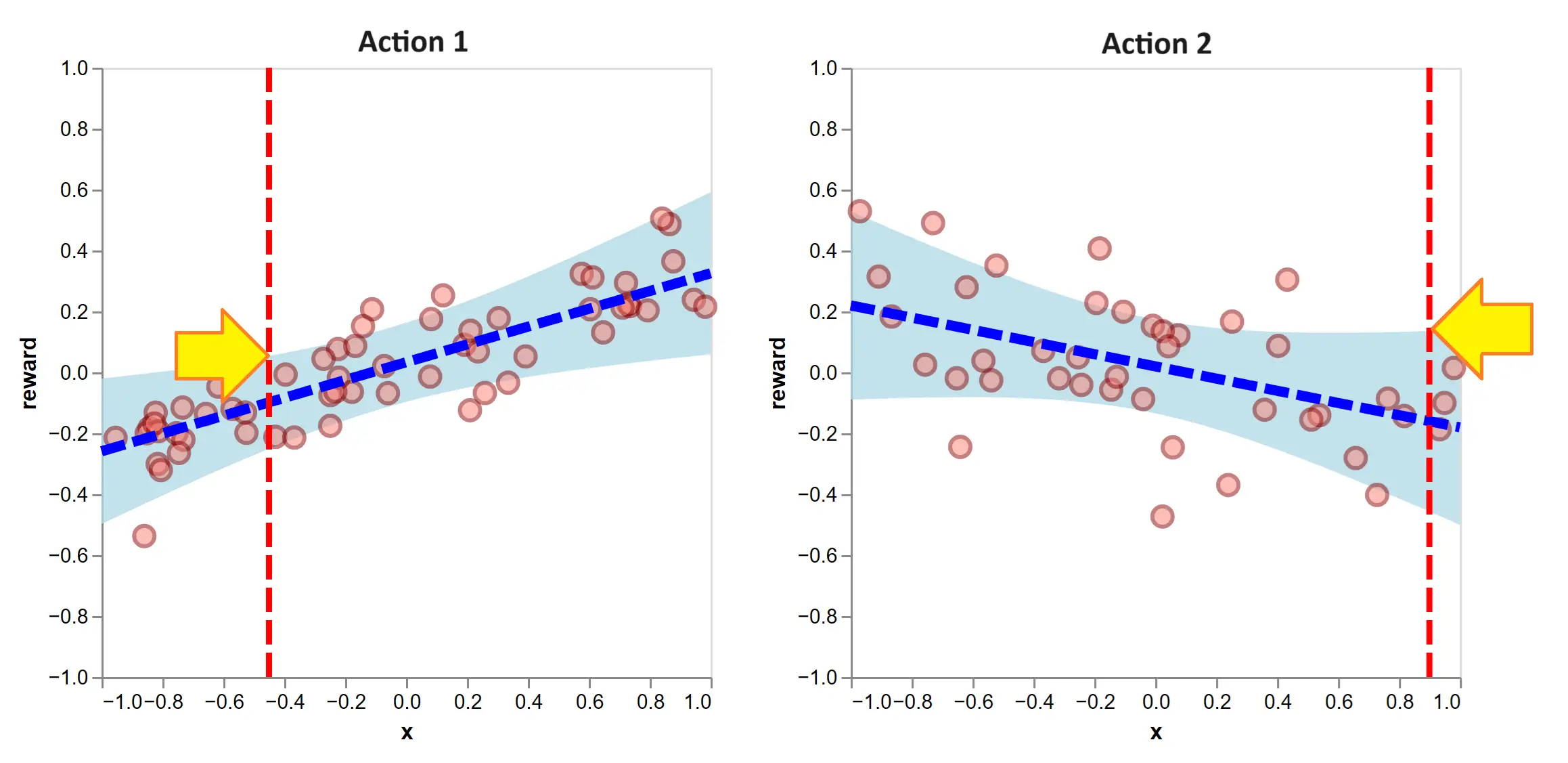 Figure 10: After 100 exploratory rounds, we fit ridge regression models. Ridge regression permits efficient calculations of confidence intervals over the expected reward. The optimism-under-uncertainty heuristic means, for the given contexts, we select the action with the higher UCB, indicated with the yellow arrows. In this case, that is to select action 2.
The UCB’s are indicated with the height of the yellow arrows. By the optimism heuristic, we select action 2 (that is, \(a_{101} = 2\)), since it has the higher UCB. This is to be ‘optimistic’ because its equivalent to believing each action’s true expected reward is at its upper confidence bound and selecting the highest. This optimism is what causes the algorithm to explore.
To clarify a point of confusion, these confidence bands are referring to the likely positions of the true expected rewards. They do not illustrate the distribution of the reward around its expectation, as was done in the first section. Notably, the action-selection rule only references the distribution of the expected reward and no other piece of the reward distribution. So if two actions had equal expected reward and equal expected reward variance but action 1 had a higher reward variance, LinUCB would be indifferent between the two. The assumption is that other differences in reward distribution are no indication of something worth learning for accruing future reward.
Further, the width of the confidence bands are scaled by a tunable hyperparameter \(\alpha > 0\). It answers the question ‘how optimistic are we?’ If \(\alpha \approx 0\), we are quick to exploit. The confidence bands are very thin and we select the highest expected reward action virtually every time. If \(\alpha\) is very large, the confidence intervals dominate the selection; we select the action we are most uncertain about.
LinUCB: the Algorithm
The previous section is illustrative, but is univariate and not quite right because LinUCB does not begin with a batch of random exploratory rounds. In LinUCB, each round balances exploration and exploitation, much like the 101-th round plotted above. In this section, we’ll discuss the algorithm generally and exactly, following the presentation in the original paper.
Let \(\mathbf{r}_{k}\) refer to the observed rewards of action \(k\) collected into a vector. Note that after 100 rounds, this vector will very likely have fewer than 100 observations, since we observe only one action’s reward per round. Next, let \(\mathbf{X}_{k}\) be a matrix with the context vectors of action \(k\) as rows. Again, this matrix is only for context vectors that were chosen5. With regularization hyperparameter \(\lambda\), the ridge regression estimate is:
\[\hat{\boldsymbol{\theta}}_k = \big(\mathbf{X}_{k}^{\top}\mathbf{X}_{k} + \lambda \mathbf{I}\big)^{-1}\mathbf{X}_{k}^{\top}\mathbf{r}_{k}\]And the estimated expected reward for action \(k\) is \(\mathbf{x}_{t, k}^{\top}\hat{\boldsymbol{\theta}}_k\). Further, when the assumptions of ridge regression hold (e.g. IID noise), we can form a confidence interval as follows. With probability at least \(1 - \delta\), we have:
\[\Big| \mathbf{x}_{t, k}^{\top}\hat{\boldsymbol{\theta}}_k - \mathbf{x}_{t, k}^{\top}\boldsymbol{\theta}_k \Big| < \alpha \sqrt{\mathbf{x}_{t, k}^{\top}\mathbf{A}_k^{-1}\mathbf{x}_{t, k}^{\phantom{\top}}}\]where \(\mathbf{A}_k = \mathbf{X}_{k}^{\top}\mathbf{X}_{k} + \lambda \mathbf{I}\) and \(\alpha = 1 + \sqrt{\ln(2/\delta)/2}\) is the width-controlling hyperparameter describe previously. Note that \(\mathbf{x}_{t, k}^{\top}\boldsymbol{\theta}_k\) is the true expected reward of action \(k\) under our assumptions.
This enables us. For every action, we can construct ranges which will contain the true expected reward with a pre-specified probability. By the optimism-under-uncertainty heuristic, we choose the action with the highest expected reward within these ranges. That is, we set:
\[a_t = \underset{k=1, \cdots, K_t}{\arg\max} \Big(\mathbf{x}_{t, k}^{\top}\hat{\boldsymbol{\theta}}_k + \alpha \sqrt{\mathbf{x}_{t, k}^{\top}\mathbf{A}_k^{-1}\mathbf{x}_{t, k}^{\phantom{\top}}}\Big)\]This expression is the generalized action-selection rule illustrated in the previous section and tells us everything we need to compute to select an action. Outside of the given context vectors and \(\alpha\), we need \(\mathbf{A}_k\) and \(\hat{\boldsymbol{\theta}}_k\). Both of these could be computed in an online fashion, updating (instead of recomputing) their values on each round.
Expanding notation slightly, if \(\mathbf{A}_k^{(t)}\) is defined for data up until round \(t\), then on each round, we perform:
\[\mathbf{A}_{a^t}^{(t)} = \mathbf{A}_{a^t}^{(t-1)} + \mathbf{x}_{t, a^t}^{\phantom{\top}}\mathbf{x}_{t, a^t}^{\top}\]Notice we are using the subscript \(a^t\) where one might expect \(k\). This says the update is only done for the selected action.
To update \(\hat{\boldsymbol{\theta}}_k\), we let \(\mathbf{b}_k = \mathbf{X}_{k}^{\top}\mathbf{r}_{k}\). So \(\hat{\boldsymbol{\theta}}_k = \mathbf{A}_k^{-1}\mathbf{b}_k\). On each round, we update:
\[\mathbf{b}_{a_t}^{(t)} = \mathbf{b}_{a_t}^{(t-1)} + r_{t, a_t}\mathbf{x}_{t, a_t}\]One could also update \(\mathbf{A}_k^{-1}\) with the matrix inversion lemma, but this may create issues of numerical stability. If the inversion creates a compute constraint, one could use the Delta rule to approximate the changes to \(\hat{\boldsymbol{\theta}}_{a_t}\).
With this, the algorithm is copied here:
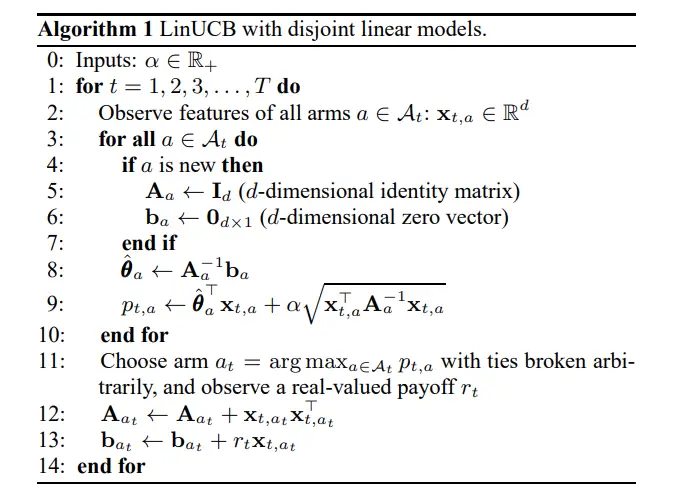 Algorithm 1 from Li (2010)
I’ll clarify some minor differences. I included the regularizing hyperparameter \(\lambda \geq 0\) that comes with ridge regression6. The adjustment to this algorithm is to replace \(\mathbf{I}_d\) with \(\lambda\mathbf{I}_d\), where \(d\) is the dimension of the associated context vector. \(\mathcal{A}_t = \{1, \cdots, K_t\}\) is the set of actions available at round \(t\). Further, this algorithm uses \(a\) where I would use \(k\), to index all actions and distinguish it from the selected action \(a_t\).
Essentially, this algorithm does what we illustrated on the 101-th round, except for all rounds and in an efficient online fashion. Here, with one simulation, we show its behavior in selecting actions, updating the distribution of expected rewards and accruing a flattening regret:
 Figure 11: Running the LinUCB algorithm using \(\lambda = 1\) and \(\alpha = .5\). Here, we show realized regret (also called pseudo regret), since it is available for a single simulation. It is defined similarly to how we defined regret, except the action selections are not averaged out. In other words, it is random since action selections depend on the random history of observations.
Running many simulations, we estimate regret, which is substantially lower than all the explore-then-exploit runs we did above.
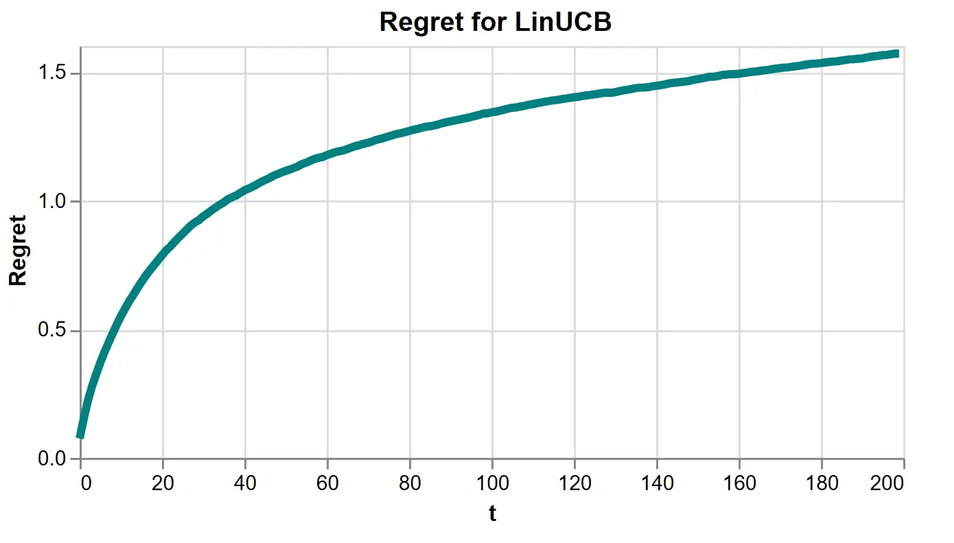 Figure 12: LinUCB’s regret estimated over 5000 simulations using \(\lambda = 1\) and \(\alpha = .5\).
If you’d like to play with the algorithm yourself, you can find the demo code here.
In Closing
This algorithm and its cousin algorithm, Algorithm 2 from Li (2010) handling the shared-features case, are strong options for applied contextual bandit problems, in my experience. They are empirically performant, interpretable, simple to code, able to handle large data, stable when training and flexible via context feature engineering. If you are considering an online7 contextual bandits algorithm, it is a fine place to start. Another good option is to reach out to us.
Also, I will mention a technical mistake of LinUCB. It was pointed out in Abbasi-Yadkori (2011) that LinUCB, among others, assumes the observations are independent across rounds. Indeed, ridge regression assumes rows are independent samples. This is not actually true. Observations depend on actions, which depend on historical observations. This technicality has implications for LinUCB performance, but it remains a safe option in practice. Because it’s an interesting complexity, I expect to explore it in a future post.
Finally, I’d like to thank Oege Dijk for his helpful feedback and commentary on this article.
References
-
L. Li, W. Chu, J. Langford and R. E. Schapire. A Contextual-Bandit Approach to Personalized News Article Recommendation. Proceedings of the 19th international conference on World wide web. April, 2010.
-
L. Zhou. A Survey on Contextual Multi-armed Bandits. arXiv:1508.03326v2. February 1, 2016.
-
Y. Abbasi-Yadkori, D. Pal and C. Szepesvari. Improved Algorithms for Linear Stochastic Bandits. NIPS. 2011.
-
Aleksandrs Slivkins. Introduction to Multi-Armed Bandits. arXiv. 2019.
-
A. Bietti, A. Agarwal and J. Langford. A Contextual Bandit Bake-off. arXiv:1802.04064v5. 2021
Something to Add?
If you see an error, egregious omission, something confusing or something worth adding, please email dj@truetheta.io with your suggestion. If it’s substantive, you’ll be credited. Thank you in advance!
Footnotes
-
If you read the post Contextual Bandits as Supervised Learning, you may recall there was one feature vector per round. That is, contextual bandits as presented there had only shared features. So, does this present two version of the contextual bandit problem? No, a single vector in each round could be a concatenation of vectors describing each action. So, separating shared features and non-shared features does not change the permissible information of the contextual bandit problem. In this post and the last, the problem is the same. However, the LinUCB algorithm has two variants which are different in this regard. This is because the calculation of uncertainty depends on where a feature is shared or not. ↩
-
In applications, we have the added complexity of selecting the functional form of the action functions. Is it linear? A neural net? Something tree-like? In my experience, real world applications are quite noisy, data constrained and nonstationary, making linear models a safe and reasonable choice.
On a technical note, the assumption that the true expected reward function belongs to a class of function from which we estimate is called realizability. For example, we assume realizability if we assume the action functions are linear and apply linear regression. In practice, realizability rarely holds exactly but is accepted as an approximation. ↩
-
The literature has several definitions of regret, so I highlight the specific one I’m using. ↩
-
To distinguish Bayesian and frequentist concepts, we should technically call these ‘credible’ intervals. However, the contextual bandit literature makes no such distinction, so I’ll continue calling them confidence intervals. ↩
-
It’s worth noting that LinUCB is throwing out all contextual vectors which weren’t selected. This is quite a bit of information, and it could be used, a la semi-supervised learning, to learn covariance information on the contextual vectors. In practice, however, it is reasonable. LinUCB quickly learns which actions are worth not selecting. To perform updates for all contextual vectors is to waste compute on actions known to yield little reward. ↩
-
There is something lost in the import of ridge regression’s \(\lambda\). In supervised learning, \(\lambda\) may be chosen via cross validation. That selection process is specific to the size of the data. Smaller data is likely to select for a larger \(\lambda\). In contextual bandits, the size of the data is not fixed, and so there is no analogous selection criteria. I suspect this may be a reason \(\lambda\) was omitted from the original algorithm. Nonetheless, it has a meaningful impact on performance, so I include it. ↩
-
Since it would be a digression and this post is long enough, I have left out the discussion of on-policy versus off-policy methods. In practice, off-policy methods are much more common. On-policy methods require the algorithm learns in live environments. Off-policy methods allow learning from historical data collected under a different policy, but it suffers degraded estimates of the policy’s performance. LinUCB, as presented, is an on-policy method but can be adapted to be off-policy. You should be aware that managing the bias and variance issues of off-policy methods is a delicate business. ↩