Summaries

The below is useful as a reference when reading the series on Probabilistic Graphical Models. It may also be useful to read the Notation Guide.

Summary of Part 1: An Introduction to Probabilistic Graphical Models

PGMs are used to represent a complex system.

We defined a complex system as a set \(\mathcal{X}\) of \(n\) random variables with a relationship we’d like to understand. We assume there exists some true but unknown joint distribution \(P\) which governs the system. We seek the ability to answer two categories of questions regarding \(P\):

1. Probability Queries: Compute the probabilities \(P(\mathbf{Y} \vert \mathbf{E}=\mathbf{e})\). That is, what is the distribution of \(\mathbf{Y}\) given some observation of the random variables of \(\mathbf{E}\)?
2. MAP Queries: Determine \(\textrm{argmax}_\mathbf{Y}P(\mathbf{Y} \vert \mathbf{E}=\mathbf{e})\). That is, determine the most likely joint assignment of one set of random variables given a joint assignment of another.

\(\mathbf{E}\) and \(\mathbf{Y}\) are arbitrary subsets of \(\mathcal{X}\). If this notation is unfamiliar, see the Notation Guide.

The idea behind PGMs is to represent \(P\) with two objects:

1. A graph: a set of nodes, one for each random variable in \(\mathcal{X}\), and a set of edges between them. Assuming a graph is to assume a set of Conditional Independence statements, which enable tractable computations.
2. Parameters: objects that, when paired with a graph and a certain rule, allow us to calculate probabilities of assignments of \(\mathcal{X}\).

Depending on these, PGMs primarily come in two flavors: a Bayesian Network (‘BN’) or a Markov Network (‘MN’).

A Bayesian Network involves a graph, denoted as \(\mathcal{G}\), with directed edges and no directed cycles. Their parameters may be specified as Conditional Probability Tables (‘CPTs’), which are, as the naming suggests, tables of conditional probabilities. They provide information to compute the right side of the Chain Rule, which states how probabilities are computed according to the BN:

\[P_{B}(X_1,\cdots,X_n)=\prod_{i=1}^n P_{B}(X_i \vert \textrm{Pa}_{X_i}^\mathcal{G})\]

where \(\textrm{Pa}_{X_i}^\mathcal{G}\) is the set of parents of \(X_i\) within \(\mathcal{G}\).

A Markov Network’s graph, denoted as \(\mathcal{H}\), is different in that its edges are undirected and it may have cycles. The parameters are a set of functions, called factors, which map assignments of subsets of \(\mathcal{X}\) to nonnegative numbers. Those subsets, labeled \(\mathbf{D}_i\)’s, correspond to complete subgraphs of \(\mathcal{H}\). We refer to the set of \(m\) factors as \(\Phi=\{\phi_i(\mathbf{D}_i)\}_{i=1}^m\).

With that, we say that the Gibbs Rule for calculating probabilities is:

\[P_M(X_1,\cdots,X_n) = \frac{1}{Z} \underbrace{\prod_{i = 1}^m \phi_i(\mathbf{D}_i)}_{\text{labeled }\widetilde{P}_M(X_1,\cdots,X_n)}\]

where \(Z\) is defined such that the probabilities sum to one.

Lastly, we recall that the Gibbs Rule may express the Chain Rule; we can always recreate the probabilities produced by a BN’s Chain Rule with a MN and its Gibbs Rule. This can be done by defining factors equivalent to the CPDs. This equivalence allows us to reason in terms of the Gibbs Rule while assured whatever we discover will also hold for BNs. In other words:

With regards to the inference algorithms we’ll cover, if a result holds for \(P_M\), it holds for \(P_B\).

Summary of Part 2: Exact Inference

Inference: The task of answering queries of a fitted PGM.

The questions are probability queries and MAP queries, as described above. Such queries have exact answers and exact inference algorithms calculate them exactly.

Doing so amounts to filtering, summing and maxing over a table, the Gibbs Table, which provides the unnormalized probabilities for all possible assignments of variables. As an example, it may look like:

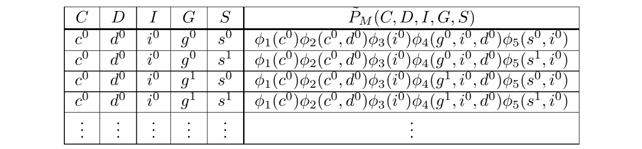The Gibbs Table \(\\\) The right column is expressed symbolically, but since the PGM is known, they may be resolved to numbers.

In general, a Gibbs Table will have exponentially many rows and so, will be too large to store.

Exact inference algorithms exploit two mechanisms to efficiently produce query answers identical to those produced with a naive calculation. Those mechanisms are:

• Factorization: The algorithms perform query transformations akin to \(ac + ad + bc + bd \rightarrow (a+b)(c+d)\), essentially seeking to multiply wherever possible, reducing the number of operations.
• Caching: A query is likely to involve redundant operations. Cleverly storing outputs enables trading memory for shortcutting computation.

One notable example is the Variable Elimnation algorithm.

Summary of Part 3: Variational Inference

Variational Inference is an approximate inference algorithm; it accept approximate answers to queries for improved efficiency. Its approach is to cast inference as an optimization problem, where the solution approximates the sought distribution but comes from a family that guarantees tractable inference.

This involves three components:

1. A space of tractable distributions: In the example covered, we considered a space of distributions whereby each is constructable as the product of univariate distirbutions.
2. A measure of dissimilarity: This measures how well a tractable distribution \(\textrm{Q}\) matches the given distribution we seek to approximate \(P_M\).
3. A search algorithm: This specifies how exactly the space of tractable distributions is searched to yield \(\hat{\textrm{Q}}\), a tractable distribution that minimizes dissimilarity and thus well approximates \(P_M\).

One is to determine the tractable space of distributions, search it to produce one, \(\hat{\textrm{Q}}\), that approximates \(P_M\) and then apply exact inference on \(\hat{\textrm{Q}}\), which is guaranteed, by the space’s design, to be efficient.

Summary of Part 4: Monte Carlo Methods

Monte Carlo methods refer to a category of approximate inference algorithms that generate samples which approximate the target distribution \(P_M\). Queries can be answered as calculations on the samples.

In particular, Markov Chain Monte Carlo (MCMC) involves generating sequences of samples \(\mathbf{x}^{(0)}, \mathbf{x}^{(1)}, \cdots, \mathbf{x}^{(t)}\) such that, beyond a certain \(t\), they may be considered samples from \(P_M(\mathbf{X})\). Such samples are of a Markov Chain, specified with transition probabilities \(\mathcal{T}(\mathbf{x} \rightarrow \mathbf{x}')\). That is, \(\mathcal{T}\) governs how \(\mathbf{x}^{(t)}\) is generated from \(\mathbf{x}^{(t-1)}\). Crucially, \(\mathcal{T}\) may be designed such that \(\mathbf{x}^{(t)}\) is effectively a sample from \(P_M(\mathbf{X})\) for large \(t\).

There are several challenges to be aware of:

• Autocorrelation: It is typical for \(\mathbf{x}^{(t)}\) and \(\mathbf{x}^{(t+d)}\) to be strongly correlated for small \(d\), meaning the set of samples are dependent. This ultimately degrades the quality of their statistical inferences.
• Computation: It is easy to specify a graph large enough, a query hard enough and an approximation strong enough that the necessary computations are infeasible. A practioner should anticipate such things before applying these methods.

Summary of Part 5: Learning Parameters of a Bayesian Network

Learning a Bayesian Network’s parameters amounts to using data to inform the Conditional Probability Distributions (‘CPDs’) of its Chain Rule:

\[P_{B}(X_1,\cdots,X_n)=\prod_{i=1}^n \underbrace{P_{B}(X_i \vert \textrm{Pa}_{X_i}^\mathcal{G})}_{\substack{\textrm{to be learned}\\\textrm{from data}}}\]

We refer to parameters, which determine the CPDs, with the vector \(\boldsymbol{\theta}\).

Learning takes the form of an optimization problem:

\[\hat{\boldsymbol{\theta}} = \textrm{argmax}_\boldsymbol{\theta} \log \mathcal{L}(\boldsymbol{\theta})\]

where:

• \(\mathcal{L}(\boldsymbol{\theta})\) is the likelihood function, giving the probability of the data \(\mathcal{D}=\{\mathbf{x}^{(i)}\}_{i=1}^w\) when it’s calculated using the Chain Rule and \(\boldsymbol{\theta}\).
• \(\hat{\boldsymbol{\theta}}\) is the maximum likelihood estimate, that which maximizes the likelihood.

In the case of a BN and complete data (no missing entries in \(\mathcal{D}\)), the log likelihood enjoys a computationally advantageous decomposition. \(\log \mathcal{L}(\boldsymbol{\theta})\) turns out to be a sum of terms which can be independently optimized. Specifically:

\[\log \mathcal{L}(\boldsymbol{\theta}) = \sum_{j=1}^n \log \mathcal{L}_j(\boldsymbol{\theta})\]

where \(j\) indexes over the \(n\) variables of \(\mathbf{X}\). Crucially, there is a subset of elements from \(\boldsymbol{\theta}\) which determines only \(\log \mathcal{L}_1(\boldsymbol{\theta})\), another subset which determines only \(\log \mathcal{L}_2(\boldsymbol{\theta})\) and so on. This means we may optimize each \(\log \mathcal{L}_j(\boldsymbol{\theta})\) independently and paste the learned sub-vectors together to form \(\hat{\boldsymbol{\theta}}\). This is a much lighter lift than optimizing all of \(\boldsymbol{\theta}\) jointly.

But this advantage is impeded with missing data. When \(\mathbf{x}^{(i)}\) contains missing values, the log likelihood necessitates a sum over all possible combinations of missing values. This couples the otherwise de-couple-able \(\log(\boldsymbol{\theta})\), as many as are included in the missing value summation.

Summary of Part 6: Learning Parameters of a Markov Network

Markov Network parameter learning is hard. To explore this, we consider a specific parameter learning task. We suppose the count of factors \(m\) and the variable subsets they map from \(\{\mathbf{D}_j\}_{j=1}^m\) are known. The goal is to learn the functions \(\{f_j(\mathbf{D}_j)\}_{j=1}^m\) of the Gibbs Rule:

\[P_M(X_1,\cdots,X_n) = \frac{1}{Z} \exp\big(\sum_{j = 1}^m f_j(\mathbf{D}_j)\big) \\\]

To turn the task of learning functions into one of learning parameters, we write \(f_j(\mathbf{D}_j)\) as a weighted sum over \(\vert \textrm{Val}(\mathbf{D}_j) \vert\) indicator functions. The weights \(\theta_j^k\) are to represent \(f_j(\mathbf{D}_j)\) for a particular assignment of \(\mathbf{D}_j\), that which is selected by the indicator \(b_j^k(\mathbf{D}_j)\):

\[f_j(\mathbf{D}_j) = \sum_{k=1}^{\vert \textrm{Val}(\mathbf{D}_j) \vert} \theta_j^k b_j^k(\mathbf{D}_j)\]

When substiting this into the Gibbs Rule, we are left with an expression:

\[P_M(X_1,\cdots,X_n) = \frac{1}{Z} \exp\big(\sum_{j = 1}^m \theta_j f_j(\mathbf{D}_j)\big)\]

where \(m\), \(\theta_j\), \(\mathbf{D}_j\) and \(f_j(\cdot)\) have been redefined for brevity. They’re defined such that the \(f_j(\cdot)\)’s are indicators, \(\theta_j\)’s are function outputs and there’s been no exclusion of learnable functions relative to the original learning objective. From this, the task is to learn \(\boldsymbol{\theta}\).

As was done in the Bayesian Network case, this comes down to a likelihood function. \(\mathcal{L}(\boldsymbol{\theta})\) gives the probability of \(\mathcal{D}\) if the probability of observed assignments is produced via the Gibbs Rule when using \(\boldsymbol{\theta}\). The learning objective may be stated as finding the MLE \(\hat{\boldsymbol{\theta}}\):

\[\hat{\boldsymbol{\theta}} = \textrm{argmax}_\boldsymbol{\theta} \log \mathcal{L}(\boldsymbol{\theta})\]

Assuming gradient based optimizer will be used, the following result is relevant:

\[\frac{\partial }{\partial \theta_j} \frac{1}{w} \log \mathcal{L}(\boldsymbol{\theta}) = \mathbb{E}_\mathcal{D}[f_j(\mathbf{D}_j)] - \mathbb{E}_{\boldsymbol{\theta}}[f_j(\mathbf{D}_j)]\]

That is, how much to nudge a \(\theta_j\) comes down to the difference between the empirical count of the associated assignments and its expected count under \(\boldsymbol{\theta}\).

Further, since \(\log \mathcal{L}(\boldsymbol{\theta})\) is concave in \(\boldsymbol{\theta}\), the following condition holds at a global maximum \(\hat{\boldsymbol{\theta}}\):

\[\mathbb{E}_\mathcal{D}[f_j(\mathbf{D}_j)] = \mathbb{E}_{\hat{\boldsymbol{\theta}}}[f_j(\mathbf{D}_j)]\quad\quad \textrm{for } j = 1, \cdots, m\]

In words, the MLE \(\hat{\boldsymbol{\theta}}\) is that which makes the expected values of \(f_j(\mathbf{D}_j)\) equal to their empirical averages observed in the data, \(\mathbb{E}_\mathcal{D}[f_j(\mathbf{D}_j)]\).

However, arriving at this point is difficult. Computing \(\mathbb{E}_{\boldsymbol{\theta}}[f_j(\mathbf{D}_j)]\) is a potentially computationally intensive inference task and it needs to be done for every gradient step. Additionally, missing data inserts an inner summation-over-all-possible-missing-value-assignments, further burdening the log likelihood compute and in fact, eliminating the concavity of \(\log \mathcal{L}(\boldsymbol{\theta})\).

Summary of Part 7: Structure Learning

Structure learning is the task of selecting a PGM’s structure such that subsequent parameter learning will produce an accurate model. In the case of a Bayesian Network, it involves selecting a DAG. In the case of a Markov Network, the structure type is more open ended. First, we note that the selection of an undirected graph is not sufficient; it leaves more to be determined before parameter learning may take place. We considered an example whereby a structure implies a choice of features, which map assignments of variable subsets to numbers. With this and assuming a log-linear form, MN parameter learning of the feature coefficients could take place.

To perform structure learning in both cases, we consider Score-Based Structure Learning. This involves scoring structures to quantify their agreement with the data and then to select the highest scoring structure found. More specifically, it involves specifying:

1. The Search Space of Structures over \(\mathcal{X}\): A point in this space corresponds to a structure (often a graph) or a set of structures.
2. A set of operators: Applying one defines how to move from one point in the search space to a neighboring point.
3. The Score Function: This measures a point’s (or structure’s) agreement with the data, most typically done using a likelihood function.
4. A Search Algorithm: This determines how the space is searched to ultimately return the final structure.

For a Bayesian Network, we were able to devise choices of the above which would approximate a DAG’s agreement with the data, would be relatively cheap to compute and could be merely updated as operators were applied. The search algorithm was a simple hill climbing algorithm, which would produce a high scoring DAG.

For a Markov Network, the task is harder. Some issues are:

• Defining the structure of a Markov Network is more open ended than in the case of a Bayesian Network.
• By our construction, the space of structures was considerably larger than the space of DAGs.
• Computing the score function involves computing the MLE, which is harder in the Markov Network case.
• The score cannot be merely incremented when operators are applied, necessitating a full computation on the consideration of every neighboring point in the space.

Lastly, we noted:

• All the above tasks are harder with missing data.
• Structure learning as presented assumes a discrete choice of structure. Considering this may not be the best approximation to nature, Bayesian Modeling Averaging allows one to average over many structures but requires a larger computation.
• We provide a short list of software to implement cousins of probabilistic graphical modeling.

---

Something to Add?

If you see an error, egregious omission, something confusing or something worth adding, please email dj@truetheta.io with your suggestion. If it’s substantive, you’ll be credited. Thank you in advance!