The Copula and 2008

In the year following the 2008 financial crisis, Felix Salmon wrote of an unusual contributing factor, the copula. It appeared a solution to a truly intractable problem, one of critical missing information in the valuation of Mortgage Backed Securities (‘MBSs’). Its elegance and ostensible plugging-of-the-hole was all that was necessary for statisticians to signoff on otherwise impossible valuations. In total, it contributed to the issuances of billions of MBSs and CDOs with perilously optimistic estimates of value and risk.

In this post, we’ll come to understand the copula mathematically, its precarious use in financial modeling and its contribution to the financial crisis. For those of us who develop models, financial or otherwise, there’s a lesson to learn:

Mathematical concepts don’t provide information regarding complex, real world systems¹. They provide mechanisms for processing observations into probable insights or predictions.

This story, one of elegant math and disastrous consequences, teaches us a suspicion of concepts masquerading as data.

The Copula

Like all posts, we’ll take an especially close look at the mathematics. Suppose we encounter the following univariate distributions:

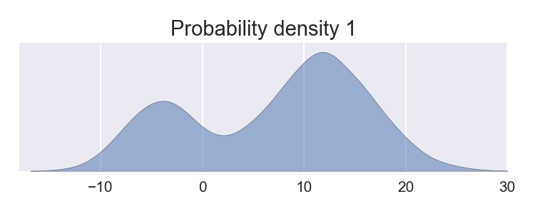
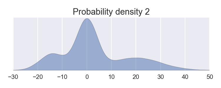
And we’re faced with a task:

Generate samples of 2D vectors from a joint distribution with a correlation of 0.8 and with the marginal distributions given above.

Critically, the joint distribution represents strictly more information than that of the marginals. Some of that information is specified with ‘0.8’. The remainder is resolved with the Gaussian assumption of the Gaussian Copula. To understand it, we need the following.

Suppose \(X\) is a continuous random variable and its cumulative density function (‘CDF’) is \(F_X(c)=\textrm{Prob}(X<c)\). We have the following:

• Probability integral transform: If \(\{x_1,x_2,\cdots,x_n\}\) are samples of \(X\), then \(\{F_X(x_1),F_X(x_2),\cdots,F_X(x_n)\}\) is uniformly distributed between 0 and 1.

• Inverse transform sampling: If \(\{u_1, u_2, \cdots, u_n\}\) are drawn from a 0-1 uniform distribution, \(\{F_X^{-1}(u_1),F_X^{-1}(u_2),\cdots,F_X^{-1}(u_n)\}\) has the distribution of \(X\).

We see, \(F_X(\cdot)\) provides a means of transforming between the uniform distribution and the distribution of \(X\).

The central idea behind the copula is as follows. Suppose we have \(d\) random variables \(X_1,X_2,\cdots, X_d\) with a joint probability density \(p(X_1,X_2,\cdots, X_d)\). The joint implies marginal distributions over each \(X_i\), which we refer to with their CDF as \(F_i(\cdot)\). If we sample a vector \([x_1, \cdots, x_d]\) from \(p(X_1, \cdots, X_d)\) and pass each element through their marginal CDF, we obtain \([F_1(x_1), \cdots, F_d(x_d)]\). If we do this \(n\) times, we obtain an \(n\)-by-\(d\) matrix \(\mathbf{U}_p\). From the probability integral transform, we know the marginal distributions of each variable, seen as the column histograms, will be uniform. But recall, these were generated from \([x_1, \cdots, x_d]\) \(\sim p(X_1, \cdots, X_d)\). This gives a marginally uniform distribution over \(d\) variables that contains the joint behavior of \(p(X_1, \cdots, X_d)\).

This is an opportunity to construct a joint distribution according to any marginal distributions we may desire. Let the CDFs of these given marginals be \(G_1(x_1), \cdots, G_d(x_d)\). We’d like to generate samples with the joint behavior of \(p(X_1, \cdots, X_d)\). To do so, we may pass each row of \(\mathbf{U}_p\) through \(G_1^{-1}(\cdot), \cdots, G_d^{-1}(\cdot)\), producing a new matrix, \(\mathbf{Y}_{p, G}\). By inverse transform sampling, we know the marginal distribution of \(\mathbf{Y}_{p, G}\) will be those of \(G_i(\cdot)\) and its joint behavior will be that of \(p(X_1, \cdots, X_d)\). Essentially:

The copula enables mixing marginal distributions with joint behavior.

With the Gaussian copula, we further assume the joint distribution is a multivariate normal distribution, enabling joint behavior to be fully specified with a correlation matrix, a relatively small thing to specify as far as \(d\)-dimensional joint distributions go. In summary, if one has a set of marginal distributions and a correlation matrix, one can generate samples from a joint distribution. A joint distribution represents more information than a set of marginals plus a correlation matrix, so the Gaussian assumption is there to fill the gap.

In the 2D example, the correlation matrix is just the 0.8 correlation. Using the copula, we can generate 2D samples:

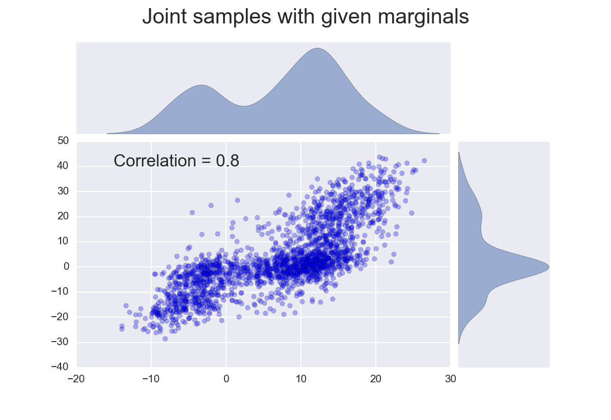
We see, the samples have the marginals as specified and a correlation of 0.8.

Valuing Mortgage Backed Securities

By the late 1990’s, bond investors had endured nearly two decades of declining bond yields, penting up demand for alternative assets. A growing product at the time were MBSs, securities offering prioritized cashflows from a large pool of mortgage holders. Risk averse investors could purchase senior ‘tranches’, receiving prioritized, safer cashflow at the cost of a lower yield. Yield hungry investors would accept a lower priority for a higher yield.

Valuing an MBS involves simulating payments from the morgage pool, passing them to securities holders according to tranching rules and discounting cash flows to produce present values². A key determinant in the valuations is risk. Over all simulations run, payments to senior security holders shouldn’t vary much, whereas they’re expected to vary considerably for less senior holders. As mentioned, this is why senior holders accept lower yields. In short:

Simulated payment variability drives price.

This variability is principally driven by the random payment and default patterns of mortgage holders. Default probabilities, repayment rates and crucially, correlations of defaults are among the required parameters and are carefully estimated from historical data.

To see the relevance of correlations, consider the extremes. If defaults are prefectly correlated, either everyone defaults in a simulation or no one does. Under this regime, there’s no incentive to be a senior holder, since senior and junior holders either both do or both don’t get paid in a simulation. Such an assumption suggests senior and junior holders should be priced the same. At the other extreme, if there is no correlation, the large and presumed diverse pool virtually guarantees senior holders will get paid, in which case they should be paid close to the risk free rate. This is to say:

Assumed correlations drive price.

But correlations are especially difficult to estimate. The direct approach involves estimating conditional probabilities, probabilities of the form:

• If group A of mortgage holders default, what is the probability group B will default? And group C? And group D? etc..
• If group A and group B default, what is the probability group C will default? And group D? etc..
• If group A, B and C default, what is the probability group D will default? And group E? etc..

In fact, this underrepresents their conditionals; they additionally depend on interest rates, consumer bank balances and wage growth, to name a few.

The difficulty arises from two facts:

1. The above presents many parameters to estimate.
2. Defaults are rare events.

In combination, this means the historical data falls pitifully short of the task. Appropriately so, this created a widespread apprehension for modeling MBSs.

David Li’s 2000 Paper

In 2000, David Li published “On Default Correlation: A Copula Function Approach,” appearantly solving the correlation problem. His recommendation had two parts:

1. To determine default correlations, use the prices of well traded credit securities that are partially driven by market expectations of default probabilities. Essentially, one is to assume default correlations can be inferred from correlations of default insurance premiums. This is dubious. Insurance premiums fluctuate according to market expectations, which frequently reveal themselves as disconnected from the underlying asset.

2. With default correlations, use a Gaussian copula to turn payers’ separate distributions of default into a joint distribution of default for all payers. This is where the Gaussian assumption does the work of filling in the otherwise unspecifiable parameters.

Together, this made the un-modelable modelable and considerably expanded the space of modelable assets. Indeed, it’s considered a driver of the infamous collateralized debt obligation (‘CDO’), whose market rose from 275 billion in 2000 to 4.6 trillion by 2006.

From here, the story is well known. Risk was repeatedly misunderstood, misrepresented and sold off to investor blind to the cash flow drivers, resulting in a historic financial crisis.

A Comment on David Li

Hindsight is 20/20; it is easy for us to wag our fingers at Li for the 2008 catastrophe. But as a matter of opinion, his public shaming isn’t in proportion to his culpability. In truth, the fault of 2008 is massively diffuse. From Richard Fuld, to statisticians, to asset managers, to regulators, to rating agencies, to banking associates, to the borrowers themselves all participated in the calamitous cascade, to varying degrees. In much the same way Li is responsible, so are the quants who applied his work. It takes no genuis to recognize its weaknesses. A properly cautious scientific community would have rejected it for filling an unknowability-hole with irrelevant data and a gaussian distribution.

I consider it a cautionary tale. Elegance is such an appeal, it biases us to over extend concepts. But complex systems aren’t bound by simply expressed ideas. They are often astronomically complex, adversarial, nonstationary, partially observed, self-referential, unmeasurable and irreducible. Acknowledging this means we limit our expectations, so we don’t suggest models do what they can’t.

References

1. F. Salmon. Recipe for Disaster: The Formula That Killed Wall Street. Wired. 2009

2. D. Li. On Default Correlation: A Copula Function Approach. Journal of Fixed Income. 2000

---

Something to Add?

If you see an error, egregious omission, something confusing or something worth adding, please email dj@truetheta.io with your suggestion. If it’s substantive, you’ll be credited. Thank you in advance!

---

Footnotes

1. A model of a complex system doesn’t qualify, since no accurate model can be developed without reference to observations. For example, this excludes general relativity. Despite its status as a set of mathematical statements pinned to physical object, its relevance distinguishing it from other sets is established only with persistent confirmatory observations. ↩

2. On a personal note, in 2013 I briefly participated in valuing shipping container securizations at BNP Paribus. Seared into memory is the excrutiating experience of translating prospectus legalese into programming logic. The need for over simplifying assumptions was clearly not limited to default correlations. ↩