The Matrix Inversion Lemma
Posted: Updated:
The matrix inversion lemma (‘MIL’) or Woodbury Matrix Identity states:
\[\big(\mathbf{A} + \mathbf{UCV}\big)^{-1} = \mathbf{A}^{-1} - \mathbf{A}^{-1}\mathbf{U}\big(\mathbf{C}^{-1} + \mathbf{V}\mathbf{A}^{-1}\mathbf{U}\big)^{-1}\mathbf{V}\mathbf{A}^{-1}\]where \(\mathbf{A}\) is an \(n\)-by-\(n\) matrix, \(\mathbf{U}\) is \(n\)-by-\(k\), \(\mathbf{C}\) is \(k\)-by-\(k\) and \(\mathbf{V}\) is \(k\)-by-\(n\). Typically, \(k \ll n\).
Despite its intimidating length, it’s actually easy to identify when to use this.
If you know1 the inverse of \(\mathbf{A}\) and would like to know the inverse of \(\mathbf{A}\) plus some low rank outer product, use the MIL.
If you have an eye for this circumstance, it’s as valuable to you as to anyone else.
An Application: Portfolio Theory
This one comes from personal experience. I’ve worked for several hedge funds and a relentless task is to predict tomorrow’s returns. To discover a performant algorithm, a large variety of candidate algorithms need to be evaluated. For this set to be large, each needs to be fast.
To see the MIL’s assist, we’ll consider a particularly simple case of backtesting an investment strategy. The data is a grid where each column provides the returns for \(n\) stocks on a particular day.
Let \(\mathbf{h}_t\) refer to a length \(n\) vector of our holdings on day \(t\). To form it optimally, we need the day’s expected returns \(\mathbb{E}[\mathbf{r}_t]\) and their covariance matrix \(\mathbb{V}[\mathbf{r}_t]\). A known result in modern portfolio theory is that the optimal unconstrained portfolio is proportional to \(\mathbb{V}[\mathbf{r}_t]^{-1}\mathbb{E}[\mathbf{r}_{t}]\). The overall size of the holdings is determined by our risk aversion, but to set that aside, we’ll seek to construct a day’s holding as:
\[\mathbf{h}_{t}=\mathbb{V}[\mathbf{r}_t]^{-1}\mathbb{E}[\mathbf{r}_t]\]But \(\mathbb{E}[\mathbf{r}_t]\) and \(\mathbb{V}[\mathbf{r}_t]\) are not known. They refer to some inaccessible ‘true’ distribution and so they must be estimated.
To do so, we will use the dirt simple concept of a rolling window with length \(w\). That is, \(\bar{\mathbf{r}}_t\) is the historical average over the past \(w\) days and \(\bar{\mathbf{C}}_t\) is the empirical covariance over the same window. The window may be pictured as:
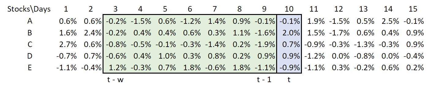 The green box of historical returns is to be used to predict returns on day \(t\).
For clarify, we will form holdings as:
\[\mathbf{h}_{t}=\bar{\mathbf{C}}_t^{-1}\bar{\mathbf{r}}_t\]Applying the MIL
From this setup, we face a problem. Everyday we must perform a slow \(\mathcal{O}(N^3)\) calculation of the inverse \(\bar{\mathbf{C}}^{-1}_t\)2. If we backtest over \(T\) days, we face an \(\mathcal{O}(TN^3)\) calculation. This is pain we can avoid.
We notice from one day to the next, \(\bar{\mathbf{C}}_t\) changes by a small amount, that of dropping one day and adding the next. If we define \(\boldsymbol{\delta}_{t}=\bar{\mathbf{r}}_{t}-\bar{\mathbf{r}}_{t-w}\), we can write:
\[\bar{\mathbf{C}}_{t+1} = \bar{\mathbf{C}}_t+\frac{1}{w}\bar{\mathbf{r}}_{t}\bar{\mathbf{r}}_{t}^{T}-\frac{1}{w}\bar{\mathbf{r}}_{t-w}\bar{\mathbf{r}}_{t-w}{}^{T}-\frac{1}{w}\bar{\mathbf{r}}_t\boldsymbol{\delta}_{t}^{T}-\frac{1}{w}\boldsymbol{\delta}_{t}\bar{\mathbf{r}}_t^{T}-\frac{1}{w^{2}}\boldsymbol{\delta}_{t}\boldsymbol{\delta}_{t}^{T}\]We are enabling an update as we slide the window:
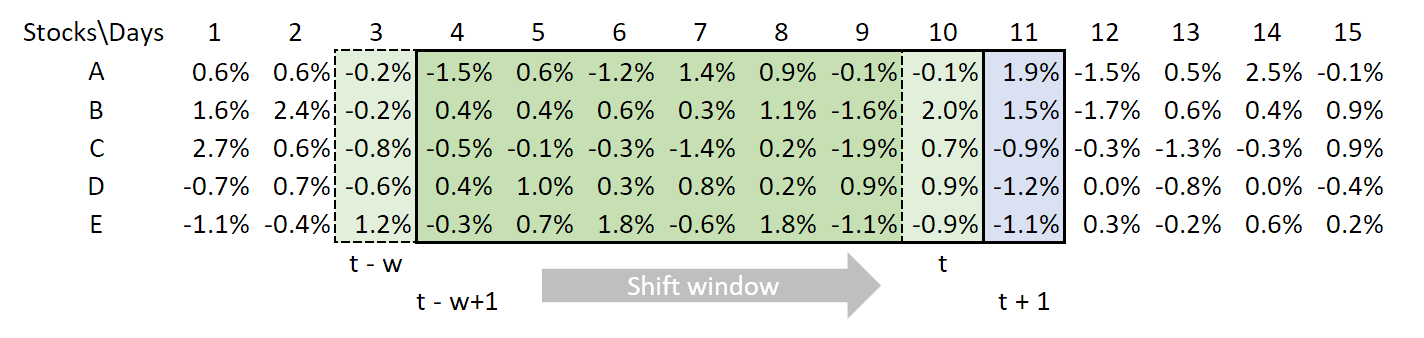 From one day to the next, the data dropped and added is small, suggesting computations can be quickened by referencing only this difference.
We notice that we’d like to compute \(\bar{\mathbf{C}}_{t+1}\) when we know \(\bar{\mathbf{C}}_t\) and their difference is an outer product. This is the circumstance to recognize!
Instead of recalculating the inverse each day, we update it with the MIL.
Before doing so, we rewrite the covariance update so the MIL may be readily applied:
\[\begin{eqnarray*} \bar{\mathbf{C}}_{t+1} & = & \bar{\mathbf{C}}_t+\frac{1}{w}\bar{\mathbf{r}}_{t}\bar{\mathbf{r}}_{t}^{T}-\frac{1}{w}\bar{\mathbf{r}}_{t-w}\bar{\mathbf{r}}_{t-w}{}^{T}-\frac{1}{w}\bar{\mathbf{r}}_t\boldsymbol{\delta}_{t}^{T}-\frac{1}{w}\boldsymbol{\delta}_{t}\bar{\mathbf{r}}_t^{T}-\frac{1}{w^{2}}\boldsymbol{\delta}_{t}\boldsymbol{\delta}_{t}^{T}\\ & = & \bar{\mathbf{C}}_t+\mathbf{L}_{t}\mathbf{W}^{-1}\mathbf{R}_{t}^{T} \end{eqnarray*}\]where \(\mathbf{L}_t\) is an \(5\)-by-\(5\) matrix , with columns of \(\bar{\mathbf{r}}_t, \bar{\mathbf{r}}_{t-w}, \bar{\mathbf{r}}_t, \boldsymbol{\delta}_{t}\) and \(\boldsymbol{\delta}_{t}\). \(\mathbf{R}_t\) is the same as \(\mathbf{L}_t\), except its third and fourth columns are switched. \(\mathbf{W}\) is a diagonal 5-by-5 matrix with a diagonal of \([w,-w,-w,-w,-w,-w^2]\). This is not too hard to hammer out after one realizes the MIL applies.
Now we may apply the MIL:
\[\begin{eqnarray*} \bar{\mathbf{C}}_{t+1}^{-1} & = & \big(\bar{\mathbf{C}}_t+\mathbf{L}_{t}\mathbf{W}^{-1}\mathbf{R}_{t}^{T}\big)^{-1}\\ & = & \bar{\mathbf{C}}_t^{-1}-\bar{\mathbf{C}}_t^{-1}\mathbf{L}_{t}\big(\mathbf{W}+\mathbf{R}_{t}^{T}\bar{\mathbf{C}}_t^{-1}\mathbf{L}_{t}\big)^{-1}\mathbf{R}_{t}^{T}\bar{\mathbf{C}}_t^{-1} \end{eqnarray*}\]This is an \(\mathcal{O}(N^2)\) operation. Assuming \(N < T\), testing one strategy will cost us \(\mathcal{O}(TN^2)\), saving us an exponent. In general, speed ups can go beyond what this suggests.
Note
As has been pointed out to me, the choice of five stocks above is a bad one. This is because that gives \(n=k=5\), which means there actually is no speed up produced. However, if we were to use more than five stocks (and suffer a slightly more complicated graphic), then there would be a speed up as described.
References
Wikipedia and appendix C of S. Boyd et al. (2004) were used for the definition and use of the MIL. H. Markowitz (1952) is a classic reference for portfolio theory. For those interested in the intersection of these concepts, chapter 4 of S. Boyd et al. (2004) discusses portfolio optimization under constraints, though it’s not related to what was covered here.
-
S. Boyd and L. Vandenberghe. Convex Optimization. Cambridge University Press. 2004.
-
H. Markowitz. Portfolio Selection. The Journal of Finance. 1952
-
Wikipedia contributors. Woodbury Matrix Identity. Wikipedia, The Free Encyclopedia.
Something to Add?
If you see an error, egregious omission, something confusing or something worth adding, please email dj@truetheta.io with your suggestion. If it’s substantive, you’ll be credited. Thank you in advance!