The Conjugate Gradient Method
Posted: Updated:
If we’re faced with a linear system \(\mathbf{Ax}=\mathbf{b}\) and are lucky enough to have \(\mathbf{A}\) be a symmetric positive definite matrix, we can exploit \(\mathbf{A}\)’s geometry to quickly navigate to the solution.
The Conjugate Gradient Method (‘CG Method’) does this from the perspective of \(\mathbf{A}\)’s eigenvalue decomposition, where spheres are discovered and an especially simple map can be drawn to the solution. To understand it, we begin by stating it precisely.
The Method in a Nutshell
The CG Method efficiently solves
\[\mathbf{Ax}=\mathbf{b}\]where \(\mathbf{A}\) is a given real symmetric positive definite matrix, \(\mathbf{b}\) is a given vector of length \(d\) and \(\mathbf{x}\) is a vector of length \(d\). The goal is to discover the \(\mathbf{x}\) that makes the equation true.
To do so, the algorithm relies on the equivalence between solving the system and finding the minimum of a certain function \(f(\cdot)\). Insights into \(f(\cdot)\)’s geometry enable fast navigation towards the minimum, where the solution is found.
What is \(f(\cdot)\)?
It’s this:
$~$f(\mathbf{x})=\frac{1}{2}\mathbf{x}^{T}\mathbf{Ax}-\mathbf{b}^{T}\mathbf{x}$~$
which is referred to as the quadratic form. Its relevance becomes clear once we inspect its gradient with respect to \(\mathbf{x}\):
$~$\nabla f(\mathbf{x})=\mathbf{Ax}-\mathbf{b}$~$
We see that if we found \(\mathbf{x}^{*}\) such that \(\nabla f(\mathbf{x}^{*})=\mathbf{0}\), it would solve the system. Further, given \(\mathbf{A}\) is symmetric and positive definite, we are assured there exists only one solution. So from this point, the goal is to minimize \(f(\cdot)\).
Contours of \(f(\cdot)\)
Let’s imagine drawing \(f(\cdot)\) starting from its minimum and expanding outward with contour lines. We ask:
What determines the set of vectors that yield the same value of \(f(\cdot)\)?
Let’s express an arbitrary point \(\mathbf{x}_{0}\) with its difference from the minimum: \(\mathbf{x}_{0}=\mathbf{x}^{*}+\mathbf{e}_{0}\). We see:
\[\begin{eqnarray} f(\mathbf{x}_{0}) & = & \frac{1}{2}(\mathbf{x}^{ * }+\mathbf{e}_{0})^{T}\mathbf{A}(\mathbf{x}^{*}+\mathbf{e}_{0})-\mathbf{b}^{T}(\mathbf{x}^{ * }+\mathbf{e}_{0})\\ & = & f(\mathbf{x}^{ * })+\frac{1}{2}\mathbf{e}_{0}^{T}\mathbf{A}\mathbf{e}_{0} \end{eqnarray}\]So the difference in value from the minimum is due entirely to \(\frac{1}{2}\mathbf{e}_{0}^{T}\mathbf{A}\mathbf{e}_{0}\).
To illustrate, say \(\mathbf{x}\) were a length-2 vector. The contours of \(f(\cdot)\) might look like:
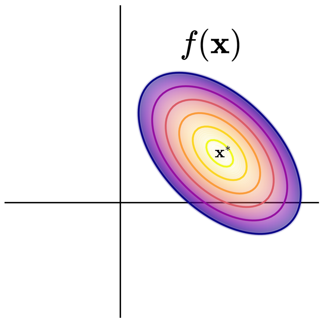 An example \(f(\mathbf{x})\) shown with contours, where the minimum value is obtained at \(\mathbf{x}^*\). The function is not plotted beyond the sixth contour line.
Here, each axis represents one of the two elements of \(\mathbf{x}\). We note two points \(\mathbf{x}_1\) and \(\mathbf{x}_2\) will yield the same output value (fall on the same contour line) if \(\mathbf{e}_{1}^{T}\mathbf{A}\mathbf{e}_{1}=\mathbf{e}_{2}^{T}\mathbf{A}\mathbf{e}_{2}\).
The Eigen-space
Due to the symmetry and positive definiteness of \(\mathbf{A}\), we can express it with its eigenvalue decomposition as:
\[\begin{eqnarray*} \mathbf{A}=\mathbf{Q}\boldsymbol{\Lambda}\mathbf{Q}^{\top} = \sum_{i}\lambda_{i}\mathbf{q}_{i}\mathbf{q}_{i}^{T} \end{eqnarray*}\]where \(\boldsymbol{\Lambda}\) is a diagonal matrix of positive eigenvalues and an eigenvalue is denoted \(\lambda_{i}\). \(\mathbf{Q}\) is a matrix of eigenvectors and an eigenvector is denoted \(\mathbf{q}_{i}\).
We know \(\mathbf{A}\) will yield \(\mathbf{q}_{i}\)’s that form a basis over \(\mathbb{R}^{d}\), so we can write \(\mathbf{e}_{0}=\sum_{i}c_{0, i}\frac{\mathbf{q}_{i}}{\sqrt{\lambda_{i}}}\). This defines a new coordinate space, the ‘eigen-space’, where for any \(\mathbf{x}_0\), we have an associated \(\mathbf{c}_0\).
One insight of the CG method is:
\(f(\cdot)\)-contours about \(\mathbf{x}^*\) correspond to circles about the origin in eigen-space.
This can be realized with:
\[\begin{eqnarray*} \mathbf{e}_{0}^{T}\mathbf{A}\mathbf{e}_{0} & = & \Big[\sum_{i}c_{0, i}\frac{\mathbf{q}_{i}}{\sqrt{\lambda_{i}}}\Big]^{T}\Big[\sum_{i}\lambda_{i}\mathbf{q}_{i}\mathbf{q}_{i}^{T}\Big]\Big[\sum_{i}c_{0, i}\frac{\mathbf{q}_{i}}{\sqrt{\lambda_{i}}}\Big]\\ & = & \sum_{i}c_{0, i}^{2} \end{eqnarray*}\]This is to say, if the eigen-coordinates, \(\mathbf{c}_1\) and \(\mathbf{c}_2\) , of two points \(\mathbf{x}_1\) and \(\mathbf{x}_2\) are the same distance from the origin, i.e. \(\sum_{i}c_{1, i}^{2} = \sum_{i}c_{2, i}^{2}\), then \(f(\mathbf{x}_1) = f(\mathbf{x}_2)\).
To illustrate, two such points along with \(\mathbf{A}\)’s eigenvectors might look like:
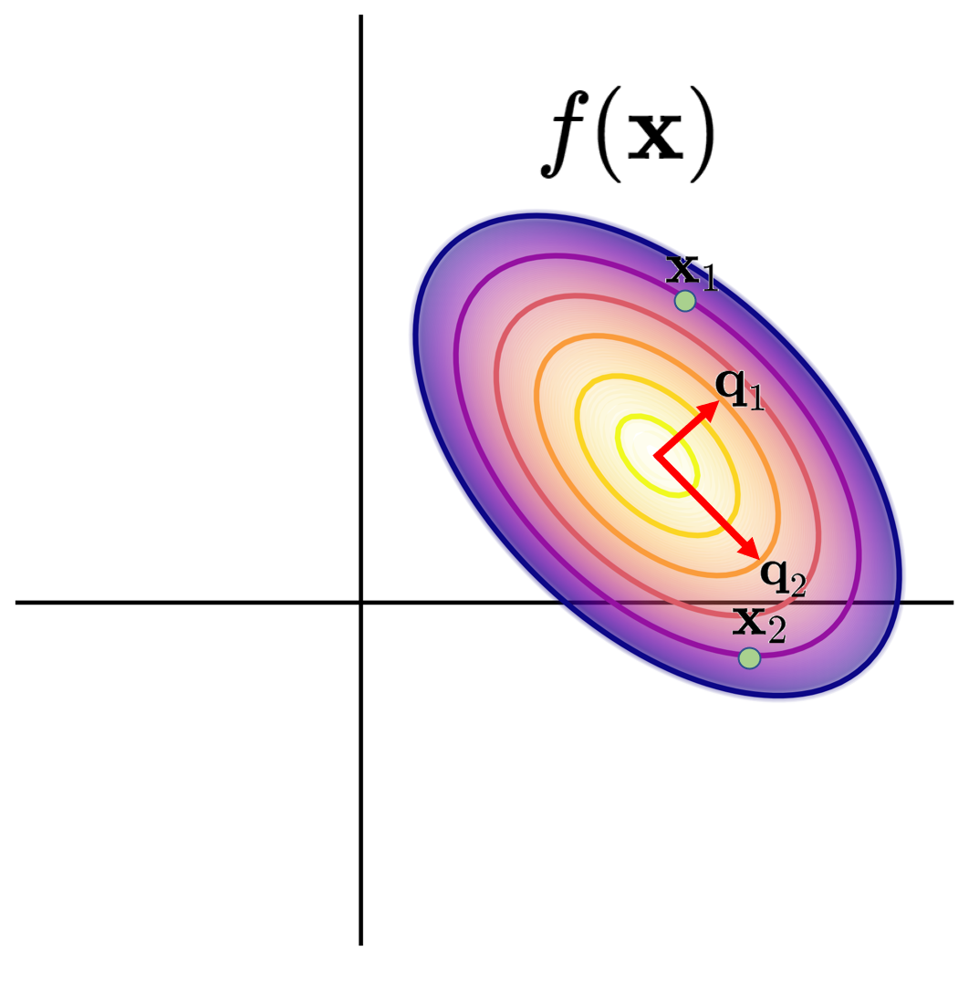 \(f(\mathbf{x})\) plotted with \(\mathbf{x}_1\) and \(\mathbf{x}_2\), where \(f(\mathbf{x}_1) = f(\mathbf{x}_2)\)
Next, we imagine the eigen-space, where the vertical and horizontal axis represent movement along \(\mathbf{q}_1\) and \(\mathbf{q}_2\), scaled down by \(\sqrt{\lambda_1}\) and \(\sqrt{\lambda_2}\) respectfully. \(\mathbf{c}_1\) and \(\mathbf{c}_2\) are the same distance from the origin, highlighting that \(f(\cdot)\)’s contours map to circles in eigen-space.
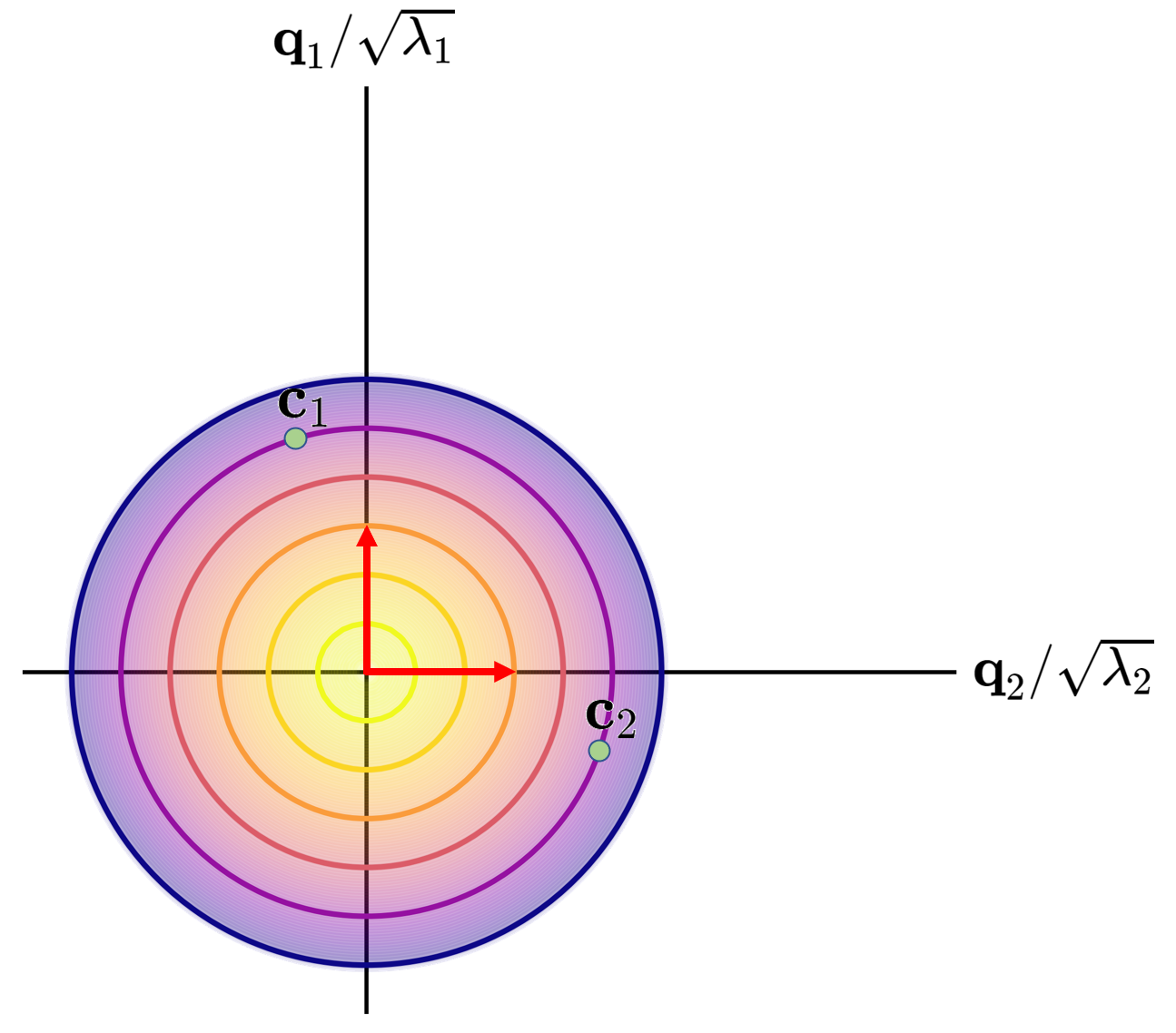 As we map \(\mathbf{x}_1 \rightarrow \mathbf{c}_1\) and \(\mathbf{x}_2 \rightarrow \mathbf{c}_2\), we realize that \(f(\cdot)\)’s contours correspond to circles in eigen-space.
Naturally, this concept generalizes to dimensions above two.
Navigating to the Solution
But how is the eigen-space’s sphere-full-ness useful?
That’s for one reason; if we move in some direction until the directional derivative in that direction is zero (equivalently, \(\nabla f(\mathbf{x})\) is orthogonal to the direction we are traveling) then at that point, the minimum falls somewhere on the plane orthogonal to that direction. That is, we are done traveling in that direction. For clarity, it can be stated slightly differently as:
In eigen-space and given a direction to travel along, we can identify a point along that direction such that the solution is on the plane orthogonal to the direction, effectively reducing the dimensionality of the problem by one.
This is the insight that makes CG so effective.
To operationalize this, we use the concept of \(\mathbf{A}\)-orthogonality.
Two points are \(\mathbf{A}\)-orthogonal if they are orthogonal in eigen-space.
Formally, vectors \(\mathbf{v}_1\) and \(\mathbf{v}_2\)1 are \(\mathbf{A}\)-orthogonal if and only if \(\mathbf{v}_{1}^{T}\mathbf{A}\mathbf{v}_{2}=0\).
The Algorithm
With these ideas, we may present the CG method. We will build a sequence of points \(\{\mathbf{x}_{0},\mathbf{x}_{1},\cdots,\mathbf{x}_{n}\}\)2 which progress towards the solution at \(\mathbf{x}_{n}\approx\mathbf{x}^{*}\), starting with \(\mathbf{x}_{0}=\mathbf{0}\). Each point will be determined with a new direction, \(\mathbf{A}\)-orthogonal to all previous directions, traveled along from the previous point. More specifically,
\[\mathbf{x}_{k}=\sum_{i=1}^{k}\alpha_{i}\mathbf{d}_{i} \quad\quad \textrm{or} \quad\quad \mathbf{x}_{k}=\mathbf{x}_{k-1}+\alpha_{k}\mathbf{d}_{k}\]Crucially, we can solve for the step sizes \(\{\alpha_{k}\}_{i=1}^{n}\). That is, using \(\mathbf{A}\mathbf{x}^*=\mathbf{b}\) and \(\mathbf{A}\)-othogonality, we can determine exactly how far to step from one point to the next, where the solution lies in the plane othogonal to the direction stepped along.
\[\begin{eqnarray*} \mathbf{Ax}_{n} & = & \sum_{i=1}^{n}\alpha_{i}\mathbf{Ad}_{i}\\ \mathbf{d}_{k}^{T}\mathbf{Ax}_{n} & = & \mathbf{d}_{k}^{T}\sum_{i=1}^{n}\alpha_{i}\mathbf{Ad}_{i}\\ \mathbf{d}_{k}^{T}\mathbf{b} & = & \alpha_{k}\mathbf{d}_{k}^{T}\mathbf{Ad}_{k}\\ \implies\alpha_{k} & = & \frac{\mathbf{d}_{k}^{T}\mathbf{b}}{\mathbf{d}_{k}^{T}\mathbf{Ad}_{i}} \end{eqnarray*}\]This is a fast means to perform line search and it’s a source of the CG method’s efficiency.
Determining Directions
The above assumes the directions \(\{\mathbf{d}\}_{i=1}^{n}\) are given. We must ask: How are they determined?
In short, they are determined as per gradient descent within the constraint that new directions are \(\mathbf{A}\)-orthogonal to old ones. That is, we determine the current negative gradient, \(\nabla f(\mathbf{x})\rvert_{\mathbf{x}=\mathbf{x}_k} = \mathbf{b}-\mathbf{Ax}_{k} = \mathbf{r}_{k}\) (called the ‘residual’), and subtract out the components that aren’t \(\mathbf{A}\)-orthogonal to the previous ones, yielding \(\mathbf{d}_{k}\).
These components can be calculated with \(\mathbf{A}\)-projections, defined as:
Computing an \(\mathbf{A}\)-projection of one vector onto another is to perform the projection in eigen-space and then to map the projection to the original space.
For two vectors \(\mathbf{v}_{1}\) and \(\mathbf{v}_{2}\), we would first write their representations as \(\mathbf{v}_{1}=\mathbf{Q}\boldsymbol{\Lambda}^{-\frac{1}{2}}\mathbf{c}_{1}\) and similarly for \(\mathbf{v}_{2}\). The projection in eigen-space is
\[\textrm{proj}_{\mathbf{c}_{2}}(\mathbf{c}_{1})=\frac{\mathbf{c}_{1}^{T}\mathbf{c}_{2}}{\mathbf{c}_{2}^{T}\mathbf{c}_{2}}\mathbf{c}_{2}\]To create the \(\mathbf{A}\)-projection, we map this to the original space by pre-multiplying by \(\mathbf{Q}\boldsymbol{\Lambda}^{-\frac{1}{2}}\):
\[\begin{eqnarray*} \textrm{proj}_{\mathbf{v}_{2}}^{\mathbf{A}}(\mathbf{v}_{1}) & = & \mathbf{Q}\boldsymbol{\Lambda}^{-\frac{1}{2}}\textrm{proj}_{\mathbf{c}_{2}}(\mathbf{c}_{1})\\ & = & \mathbf{Q}\boldsymbol{\Lambda}^{-\frac{1}{2}}\frac{\mathbf{c}_{1}^{T}\mathbf{c}_{2}}{\mathbf{c}_{2}^{T}\mathbf{c}_{2}}\mathbf{c}_{2}\\ & = & \mathbf{Q}\boldsymbol{\Lambda}^{-\frac{1}{2}}\frac{\mathbf{v}_{1}^{T}\mathbf{A}\mathbf{v}_{2}}{\mathbf{v}_{2}^{T}\mathbf{A}\mathbf{v}_{2}}\mathbf{c}_{2}\\ & = & \frac{\mathbf{v}_{1}^{T}\mathbf{A}\mathbf{v}_{2}}{\mathbf{v}_{2}^{T}\mathbf{A}\mathbf{v}_{2}}\mathbf{v}_{2} \end{eqnarray*}\]This enables us to solve for \(\mathbf{d}_{k}\), as described earlier:
\[\begin{eqnarray*} \mathbf{d}_{k} & = & \mathbf{r}_{k}-\textrm{proj}_{\{\mathbf{d}_{1},\cdots,\mathbf{d}_{k-1}\}}^{\mathbf{A}}(\mathbf{r}_{k})\\ & = & \mathbf{r}_{k}-\sum_{i=1}^{k-1}\frac{\mathbf{r}_{k}^{T}\mathbf{A}\mathbf{d}_{i}}{\mathbf{d}_{i}^{T}\mathbf{A}\mathbf{d}_{i}}\mathbf{d}_{i} \end{eqnarray*}\]In Summary
To summarize, we perform gradient descent, but apply a correction that ensures new directions are \(\mathbf{A}\)-orthogonal to previous ones traveled along. Doing this ensures we never undo the work of previous steps. Using the eigenvalue decomposition of \(\mathbf{A}\), projections in eigen-space and \(\mathbf{A}\mathbf{x}^* = \mathbf{b}\), we can sequentially determine these directions and exactly how far to step along each one. More procedurally, the algorithm takes the following form.
Start at an initial point and repeat the following one step procedure:
- Calculate the residual.
- Subtract out the \(\mathbf{A}\)-projection of the residual onto previously traveled directions, yielding a direction.
- Solve for the step size along that direction and take that step.
The algorithm ends when the residual is sufficiently small3 and we have effectively solved the system.
More generally, we can appreciate the CG method as one which exploits the geometric properties of a symmetric, positive definitive matrix \(\mathbf{A}\). This is done by thinking in \(\mathbf{A}\)’s eigen-space, where the solution lies at the center of a sphere. Due to the properties of a sphere, we can travel quickly to the center.
References
-
J. R. Shewchuk. An Introduction to the Conjugate Gradient Method Without the Agonizing Pain. Carnegie Mellon University, 1994.
-
R. Barrett, et al. Templates for the Solution of Linear Systems: Building Blocks for Iterative Methods. SIAM. 1994.
Something to Add?
If you see an error, egregious omission, something confusing or something worth adding, please email dj@truetheta.io with your suggestion. If it’s substantive, you’ll be credited. Thank you in advance!
Footnotes
-
We introduce the notation of “\(\mathbf{v}\)” to say that this definition holds for any vector. This is to differentiate it from \(\mathbf{x}\) and \(\mathbf{e}\) notation used earlier, which implied their relationship. ↩
-
To avoid confusion, \(\{\mathbf{x}_{0},\mathbf{x}_{1},\cdots,\mathbf{x}_{n}\}\) now refers to a sequence of points on the path to the solution. It does not refer to an arbitrary set of points or a set of points that yield the same \(f(\cdot)\)-output, as earlier notation suggested. ↩
-
In practice, the algorithm looks a bit different from how it has been explained. The differences result from computational short cuts that aren’t relevant to the idea behind the CG method. ↩