Motivating the Gini Impurity Metric

The Gini impurity metric is used to form a decision tree, a hierarchy of rules used to predict a target variable from feature variables. Rules are akin to “If the height is over 6-feet, the person is likely a male”. One applied to the Iris dataset looks like:

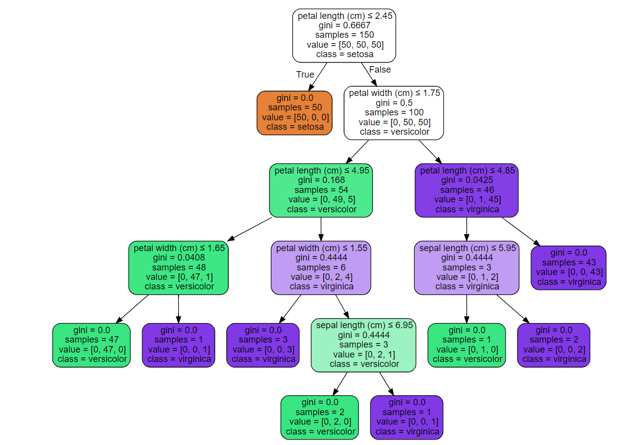A decision tree to predict the species of flower. Source

More specifically, Gini impurity is a metric to determine which variables to split on and the split locations. It’s the quantifier dictating the tree’s shape. As such, it’s crucial to understand to interpret what a decision tree is actually doing.

To form this intuition, we’ll build up the metric incrementally. This will show the Gini impurity as a natural destination, following from a goal and reasonable steps in its pursuit.

What’s the goal?

Like many machine learning tasks, it’s prediction. Suppose we’re given the following data:

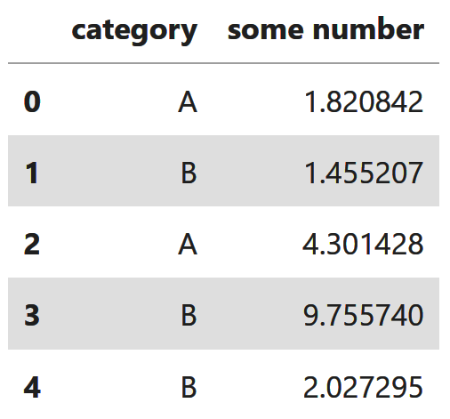
The goal is to predict the category given some number.

We begin by inspecting the histogram, colored by category:

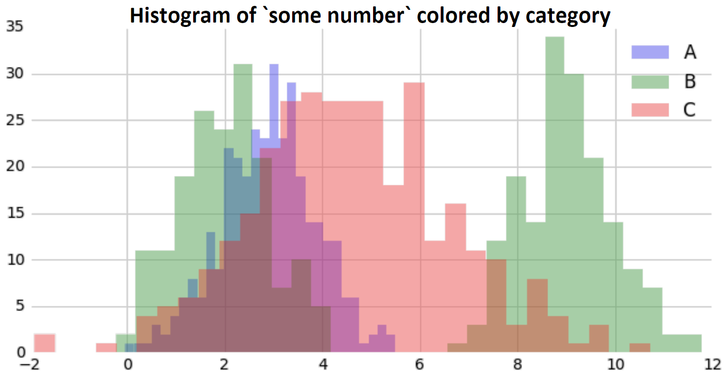
This inspires a simple idea for prediction. Divide the data along the axis, creating two sets that are pure, meaning they are maximally full of a single category. This defines two regions, where a simple prediction rule can be applied in each: predict the most common category.

To do that, we first need to answer the following.

How is a set’s purity measured?

Let’s consider a set \(\mathcal{S}_2\) with two categories:

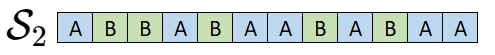
We’d like an impurity metric, something that is low if \(\mathcal{S}_2\) is pure and high when it’s impure. Something obviously useful is the fractions:

$~$ p_A = \frac{\textrm{Number of As}}{\textrm{Number of As and Bs}} $~$ $~$ p_B = \frac{\textrm{Number of Bs}}{\textrm{Number of As and Bs}} $~$

From here, one might recommend \(p_A\) as a measure of impurity. It’s low when the set is full of \(B\) (good), but high when it’s full of \(A\) (not good).

So we need something symmetric. An alternative is:

$~$ M_2(\mathcal{S}_2)=p_A\cdot p_B = p_A\cdot (1-p_A) $~$

Does this metric \(M_2\) do what we want? As a function of \(p_A\):

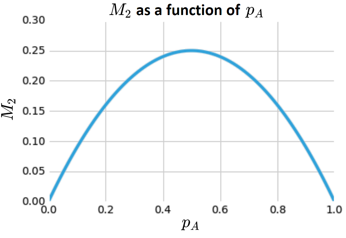
This is high when we have an even mixing and low otherwise, precisely what we want.

But what if we have more than two categories? E.g.:

This is harder. We could try:

$~$ p_A\cdot p_B \cdot p_C $~$

But a problem arises. If we have the max-impurity split of a \([\frac{1}{3},\frac{1}{3},\frac{1}{3}]\), this tops out at \(\frac{1}{27}\). When we only had \(A\)’s and \(B\)’s, it topped out at \(\frac{1}{4}\). How have we gone down in impurity by adding a new category? It should go up. More concretely, if we have \(k\) categories, then the metric should increase as \(k\) increases, in the case of the max-impurity split of \([\frac{1}{k},\frac{1}{k},\cdots,\frac{1}{k}]\). However, it shouldn’t increase indefinitely. Presumably the difference in impurity due to adding the trillionth category should be very small. In other words, it should level out.

To capture this, we should think of a function of \(k\) that has this behavior. If we’re clever, we’d guess:

\[f(k) = \sum_{i=1}^k \frac{1}{k}\big(1-\frac{1}{k}\big)\]

Which looks like:

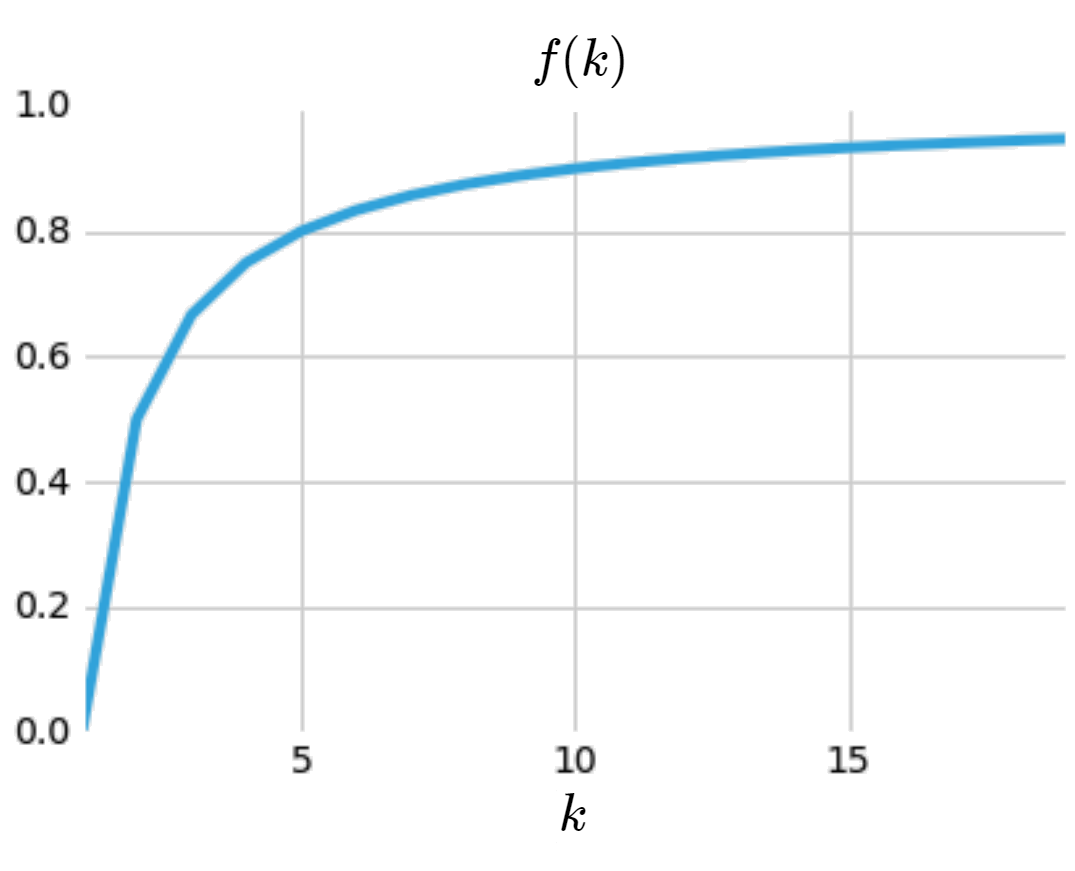
This has the intended behavior; it’s monotonically increasing but with a diminishing effect.

Next, how can we combine this with \(M_2\)? A natural combination is:

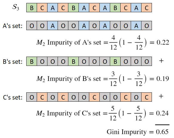
\[M(\mathcal{S}_3) = p_A\cdot (1-p_A) + p_B\cdot (1-p_B) + p_C\cdot (1-p_C)\]

And this is the Gini impurity metric. It tracks impurity and increases with diminishing returns as we add categories. Note that if we had \(k\) categories instead of three, the expression would expand to have \(k\) terms.

For a different perspective, we are effectively making a new set for each category, applying the \(M_2\) metric and summing the results:

Gini for decision trees

Now we have a metric that’ll evaluate a split point; if we drop a random split point, we’ll get impurity measures on either side:

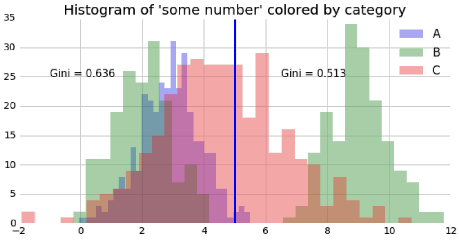
If we take the weighted average on either side, we can combine this into one number. This allows us to evaluate all split points and to select the best, lowest impurity one:

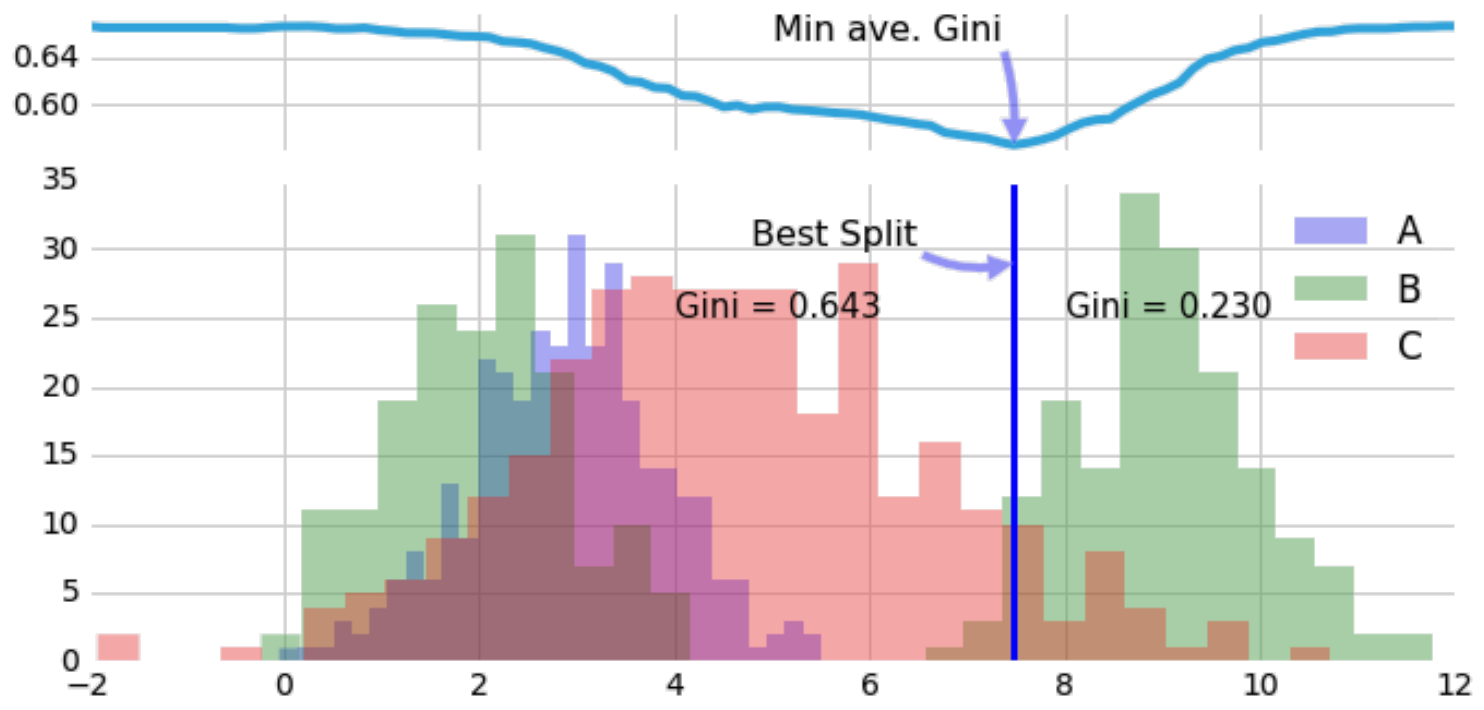
This is how we find the best split point. Subsequently, we apply the predict-most-common-category rule depending on which side a point falls.

From here, split points are applied recursively, where the variable to split along is determine as that which offers the greatest gain in purity. Ultimately, a decision tree is surfacing rectangular regions with low Gini impurity. From the above, low Gini impurities implies high purity with a small number of categories.

References

1. T. Hastie, R. Tibshirani and J. H. Friedman. The Elements of Statistical Learning: Data Mining, Inference, and Prediction 2nd ed. New York: Springer. 2009.

2. Scikit Learn contributors. Scikit-Learn Documentation: Decision Trees

---

Something to Add?

If you see an error, egregious omission, something confusing or something worth adding, please email dj@truetheta.io with your suggestion. If it’s substantive, you’ll be credited. Thank you in advance!