Part 5: Learning Parameters of a Bayesian Network
Posted: Updated:
So far, we’ve assumed we’re given a PGM with fitted parameters. Now we’ll discuss the principles for learning those parameters from data for one type of PGM, the Bayesian Network (‘BN’). We’ll begin in an idealized world of complete data to study a core object of learning, the likelihood function. Then we’ll relax the complete assumption and note the consequences. We’ll finish with practical challenges to contextualize what’s been learned.
Before proceeding, it may help to review the Notation Guide, the Part 1 summary and the Part 2 summary.
The Starting Point and Goal
The parameters of a Bayesian Network determine its Conditional Probability Distributions1 (‘CPDs’), which can produce the probability of every variable assignment given the assignment of its parents, according to the BN graph \(\mathcal{G}\).
The goal is to learn these parameters from data, which will take the form of some, at least partial, observations of the system’s variables, \(\mathcal{X}\). To start, we’ll assume the observations are complete, meaning a sample of data includes an observation for every variable of \(\mathcal{X}\).
To begin, we introduce notation. Suppose \(\mathbf{X} = \mathcal{X}\) and we have \(w\) observations of \(n\) discrete random variables, written as \(\mathcal{D}=\{\mathbf{x}^{(i)}\}_{i=1}^w\). To repeat, completeness means no entries of an \(\mathbf{x}^{(i)}\) are missing. Such data can be imagined as:
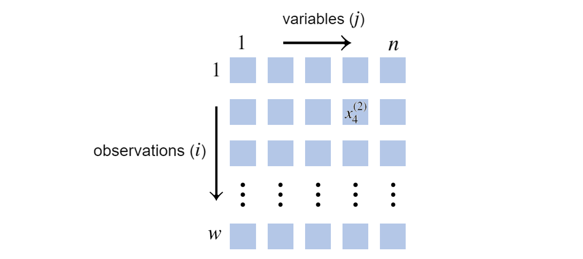 \(w\) observations of \(n=5\) variables \(\\\) Blue squares indicate discrete values, unspecified in this depiction.
For example, if this were to represent the Student Bayesian Network, one observation might be:
\[\mathbf{x}^{(1)}=[i^0,d^1,g^1,s^0,l^1]\]To summarize:
The goal is to use the above grid of data, \(w\) observations of a system of \(n\) random variables \(\mathcal{X}\), to form CPDs, assuming a given Bayesian Network graph \(\mathcal{G}\).
The Likelihood Function
The approach will rely on the likelihood function, a function of the parameters, labeled collectively as \(\boldsymbol{\theta}\), that quantifies how likely \(\mathcal{D}\) is according to \(\boldsymbol{\theta}\). It is computable from the CPDs and is labeled as:
\[\mathcal{L}(\boldsymbol{\theta})\]Regularization considerations aside, we assume the best parameters are those which maximize the likelihood. Such parameters, labeled \(\hat{\boldsymbol{\theta}}\), are called the Maximum Likelihood Estimate (‘MLE’). We may restate our goal as finding \(\hat{\boldsymbol{\theta}}\).
Since a \(\log\) transform turns products into sum and an argmax of \(\mathcal{L}(\boldsymbol{\theta})\) is an argmax of \(\log \mathcal{L}(\boldsymbol{\theta})\), we will work with latter. Using the BN Chain Rule, it can be written:
\[\log \mathcal{L}(\boldsymbol{\theta}) = \sum_{i=1}^w \sum_{j=1}^n \log P_{B}(X_j=x^{(i)}_j \vert \textrm{Pa}_{X_j}^\mathcal{G}=\mathbf{x}^{(i)}_{\textrm{Pa}_{X_j}^\mathcal{G}})\]This states we can evaluate the data’s log likelihood according to \(\boldsymbol{\theta}\) with a summation over observations and rows. Implicit in the expression is that \(\boldsymbol{\theta}\) specifies the CPDs, which by definition give us the \(P_{B}(\cdot \vert \cdot)\) information. To illustrate, we’ll compute it for a data sample using the Student example: \(\mathbf{x}^{(1)}=[i^1,d^0,g^2,s^1,l^0]\). That is:
\[\small \begin{align} \sum_{j=1}^n \log P_{B}(X_j=x^{(1)}_j \vert \textrm{Pa}_{X_j}^\mathcal{G}=\mathbf{x}^{(1)}_{\textrm{Pa}_{X_j}^\mathcal{G}})&=\log P_B(i^1)+\log P_B(d^0)\\ & \phantom{=} + \log P_B(g^2 \vert i^1,d^0) + \log P_B(s^1 \vert i^1)+\log P_B(l^0 \vert g^2)\\ & = \log 0.3+ \log 0.6+ \log 0.08+ \log 0.8+ \log 0.4\\ & \approx -5.38 \\ \end{align}\]Pictorially, we calculated the portion of \(\log \mathcal{L}(\boldsymbol{\theta})\) corresponding to the first row of \(\mathcal{D}\):

Maximizing \(\log \mathcal{L}(\boldsymbol{\theta})\) with Complete Data
Complete data eases the search for \(\hat{\boldsymbol{\theta}}\). To see this, we flip the order of the summation signs and label:
\[\begin{align} \log \mathcal{L}(\boldsymbol{\theta}) & = \sum_{j=1}^n \overbrace{\sum_{i=1}^w \log P_{B}(X_j=x^{(i)}_j \vert \textrm{Pa}_{X_j}^\mathcal{G}=\mathbf{x}^{(i)}_{\textrm{Pa}_{X_j}^\mathcal{G}})}^{\log \mathcal{L}_j(\boldsymbol{\theta})} \\ & = \sum_{j=1}^n \log \mathcal{L}_j(\boldsymbol{\theta}) \end{align}\]For example (not the Student example), if \(\textrm{Pa}_{X_3}^\mathcal{G}=\{X_4,X_5\}\), then computing \(\log \mathcal{L}_3(\boldsymbol{\theta})\) would involve the following data:
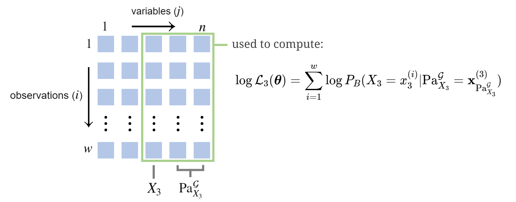
The advantage of this reframing comes with the following fact, ultimately a consequence of a BN’s Conditional Independence properties:
\(\log \mathcal{L}_j(\boldsymbol{\theta})\) depends only on a subset of \(\boldsymbol{\theta}\), those which determine \(P_{B}(X_j \vert \textrm{Pa}_{X_j}^\mathcal{G})\). We label this subset \(\boldsymbol{\theta}_{X_j \vert \textrm{Pa}_{X_j}^\mathcal{G}}\).
This means we can optimize \(\log \mathcal{L}_j(\boldsymbol{\theta})\) independently; we determine the best \(\hat{\boldsymbol{\theta}}_{X_j \vert \textrm{Pa}_{X_j}^\mathcal{G}}\) for each \(j\) and paste them together to get \(\hat{\boldsymbol{\theta}}\). The best choice of one has no effect on the best choice for another.
This is a major advantage when confronting the curse of dimensionality. It can be closely analogized as the difference between facing an optimization of 100 variables and facing 100 optimizations of a single variable each; everyone would prefer the latter!
Further, suppose \(\boldsymbol{\theta}\) specifies the CPDs by listing the table elements; they are CPTs. In this case, there’s no need to run an optimization for each \(\log \mathcal{L}_j(\boldsymbol{\theta})\). Rather, we can compute the answer directly from the data; the answer is the \(\hat{\boldsymbol{\theta}}\) which corresponds to the empirical CPTs. This amounts to computing a variable’s parameters as merely the proportion of each discrete value observed in the data, conditional on the assignment of the variable’s parents. In short, no costly optimization is necessary; merely counting observations yields the MLE.
Missing Data
If we have missing data, we have to adjust \(\mathcal{L}(\boldsymbol{\theta})\) to account for all possible ways the missing data could be. Suppose we come across:
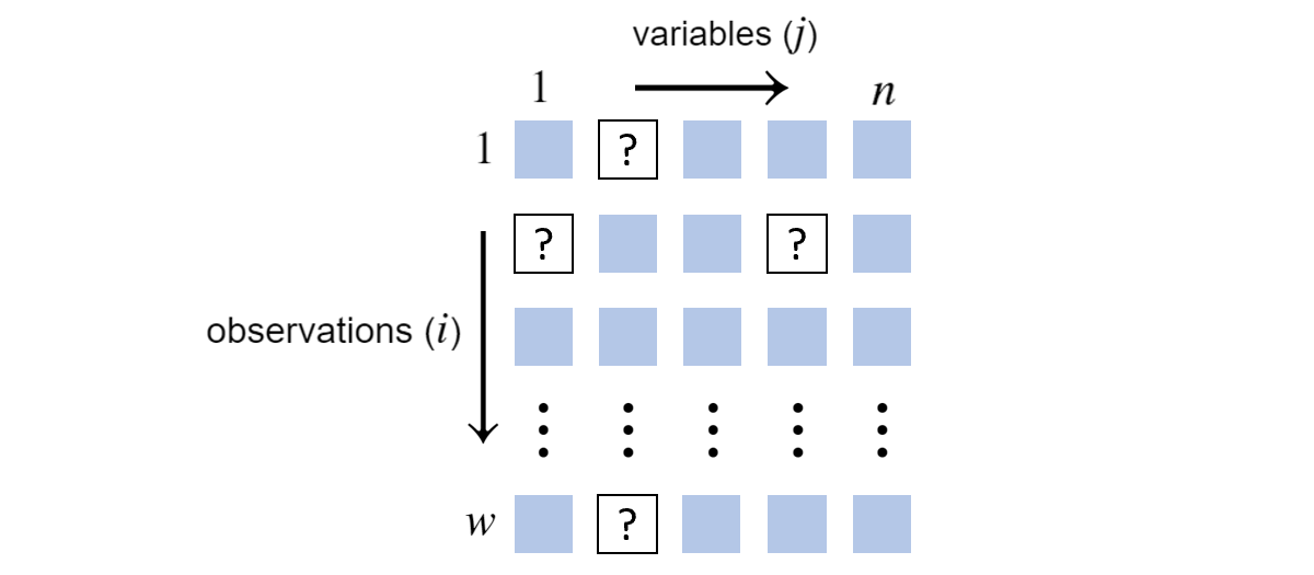 \(w\) observations of \(n=5\) variables with missing values
Suppose the placement of the missing values doesn’t depend on the random variable values. They are missing completely at random. This isn’t a realistic assumption, but the alternative would take us far afield from this presentation2.
For each row, we must consider all possible joint assignments that are consistent with the observation. In other words, we need to consider all combinations of hidden value assignments.
More precisely, let \(h(i)\) be the number of possible joint assignments to the missing variables at row \(i\). Looking at the above grid, if \(\textrm{Val}(X_1)\) has three elements and \(\textrm{Val}(X_4)\) has four elements, \(h(2)=3 \times 4 = 12\). Further, suppose \(k\) indexes over these possible combinations and \(\mathbf{x}^{(i),k}\) is \(\mathbf{x}^{(i)}\) but with the \(k\)-th combination plugged in. The likelihood function becomes3:
\[\mathcal{L}(\boldsymbol{\theta}) = \prod_{i=1}^w \sum_{k=1}^{h(i)}\prod_{j=1}^n P_{B}(X_j=x^{(i),k}_j \vert \textrm{Pa}_{X_j}^\mathcal{G}=\mathbf{x}^{(i),k}_{\textrm{Pa}_{X_j}^\mathcal{G}})\]This shows the likelihood of a data sample involves summing the products corresponding to each possible combination of hidden values. The summation is a serious problem, as the log likelihood becomes:
\[\log \mathcal{L}(\boldsymbol{\theta}) = \sum_{i=1}^w \log \big(\sum_{k=1}^{h(i)}\prod_{j=1}^n P_{B}(X_j=x^{(i),k}_j \vert \textrm{Pa}_{X_j}^\mathcal{G}=\mathbf{x}^{(i),k}_{\textrm{Pa}_{X_j}^\mathcal{G}})\big)\]Symbolically, the summation blocks the log from turning the inner most product into a sum. We’re forced to multiply across a row and we must do so for all possible combinations of hidden values. This may be pictured as:
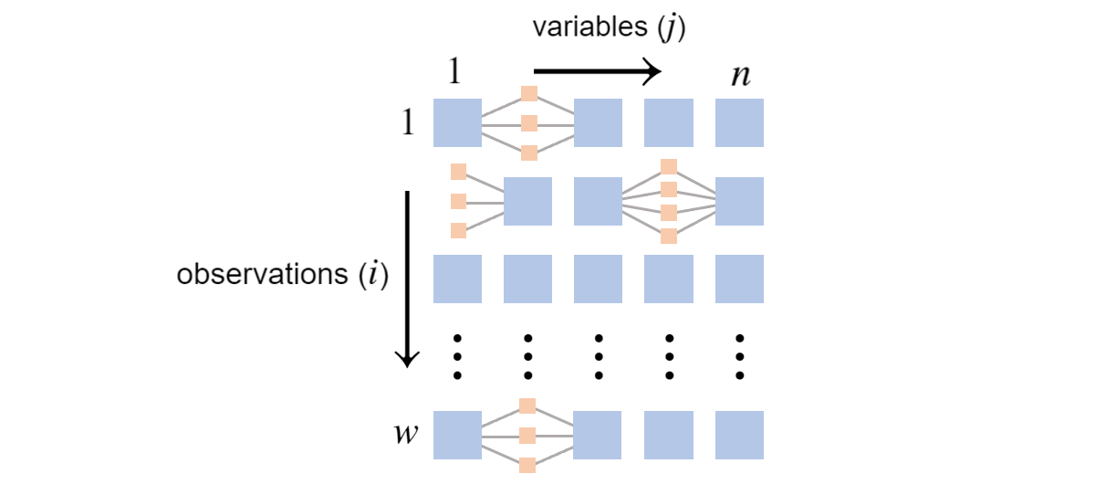
The small tan boxes represent potential hidden values. The difficulty is the log likelihood involves summing over products, one for every path through the tan boxes. In the second row, there are twelve paths. The count of paths is exponential in the number of hidden values, potentially creating a significant computational burden.
But we’re not without solutions. Missing data complicates the objective function, but it may still be optimized. Stochastic gradient descent could be used, whereby we would merely sample from all hidden combinations. Further, the expectation-maximization algorithm could be used, as it is specially designed to handle missing data. See section 4.2.7.5 of Murphy (2023) for a detailed explanation. Lastly and most simply, we may drop all non-complete observations.
Learning in Practice
The above is to present the parameter learning mechanics in the discrete variable Bayesian Network case. What is primary is the log likelihood’s separability across variables and how this separability is prevented with missing data.
But the reality of learning a BN comes with challenges unspecific to the BN case:
- How should the CPDs be parameterized? A CPT, a parameterization where \(\boldsymbol{\theta}\) lists the probability of every child assignment given every joint assignment of the parents, will be exponentially long, making it unmanageable and impossible to estimate.
- Which learning algorithm should be used and how does it interact with the choice of parameterization?
- How should regularization be done? That is, how should the log likelihood be augmented to prevent overfitting? This is especially important since counts conditional on all joint assignments of parents will have many zeros, most of which are poor predictions.
- How should the fitted parameters be evaluated? How much hold out data should be used in the evaluation?
This sampling of questions is to highlight the width of the problem and show most of it, as it doesn’t concern the BN case, falls outside what this explanation seeks to do.
The Next Step
Given the questions answered above, it’s natural to ask the same thing of a Markov Network:
Otherwise, we consider the final task:
References
-
D. Koller and N. Friedman. Probabilistic Graphical Models: Principles and Techniques. MIT Press. 2009.
-
K. Murphy. Probabilistic Machine Learning: Advanced Topics. MIT Press. 2023.
Something to Add?
If you see an error, egregious omission, something confusing or something worth adding, please email dj@truetheta.io with your suggestion. If it’s substantive, you’ll be credited. Thank you in advance!
Footnotes
-
In previous posts, we referenced Conditional Probability Tables, where every child assignment probability for every joint assignment of parents is listed in a table. When modeling, it is unlikely we’d use this representation. Rather, we’d use assumptions that allow us to compute probabilities using \(\boldsymbol{\theta}\). These assumptions are called the choice of parameterization. For example, using a logistic regression vs a neural network is a choice of parameterization. The choice of parameterization is important, but too broad of a subject for us to explore here. ↩
-
In such a case, we’d have to build the observational mechanism into the graph and the likelihood function. This complicates both of them, but doesn’t change the core of our presentation. It’s effectively just an extended graph. ↩
-
It follows from an application of the law of total probability, where conditioning is done on every joint assignment of hidden variables. ↩