Part 4: Monte Carlo Methods
Posted: Updated:
In Part 2, we defined:
Inference: The task of answering queries of a fitted PGM.
Monte Carlo methods are an approximate approach to this task. They generate answers as a set of samples approximating the sought distribution. Notably, they enjoy a generality unlike exact inference and variational inference. With exact algorithms, the cost of exactness is the limited size of the graph. Variational algorithms aren’t under the same limitation, but require additional specifications; one must design the tractable search space and how to search it. This friction inevitably constrains the range of applicable graphs. Monte Carlo methods, on the other hand, don’t require such specifications and enjoy applicability to a larger range, giving them a strong appeal.
However, the core difficulty has not vanished, but merely shifted, albeit to a place some find easier to manage. Broadly, we encounter issues of convergence and independence. Do the samples strongly approximate the distribution we seek? How should samples be generated such that they do? How long should simulations run? Which samples may be considered independent? To address these, we have diagnostic tools, evaluations and heuristics. In totality, these methods demand a specialized sampling-wrangling skillset where the degree of skill required depends on the model queried.
Before proceeding, it may help to review the Notation Guide, the Part 1 summary and optionally, the Part 2 summary.
The Starting Point
We are given a Markov Network (‘MN’), one which might be the converted form of a Bayesian Network. Specifically, we receive a graph \(\mathcal{H}\) and a set of factors \(\Phi\). We are interested in the distribution of a subset of random variables, \(\mathbf{Y} \subset \mathcal{X}\), conditional on an observation of other random variables \(\mathbf{E}=\mathbf{e}\).
We will accept the answer in terms of samples, \(\mathbf{y}\)’s, that approximately track \(P(\mathbf{Y} \vert \mathbf{E}=\mathbf{e})\). That is, obtaining such samples constitutes an ability to answer both probability and map queries.
Regarding Conditioning
We begin with a simplifying statement on conditioning. Recall an idea from part 2; inference in a MN conditional on \(\mathbf{E}=\mathbf{e}\) gives the same answer as unconditional inference in a reduced MN. Its graph is labeled \(\mathcal{H}_{ \vert \mathbf{e}}\) and its factors are labeled \(\Phi_{ \vert \mathbf{e}}\). It turns out \(\mathcal{H}_{ \vert \mathbf{e}}\) is \(\mathcal{H}\) but with all \(\mathbf{E}\) nodes and any edges involving them deleted. \(\Phi_{ \vert \mathbf{e}}\) is the set of factors \(\Phi\) but with \(\mathbf{E}=\mathbf{e}\) fixed as an input assignment. This is to say:
If we can do unconditional inference, we can do conditional inference
granted we perform the aforementioned graph and factor adjustments. For cleanliness, we’ll drop the ‘\(\vert \mathbf{e}\)’ on the graph and factor notation and assume the conditioning adjustments have been made.
Markov Chain Monte Carlo
Stated simply:
Markov Chain Monte Carlo (‘MCMC’) involves sequentially sampling \(\mathbf{y}\)’s such that, eventually, they are distributed like \(P_M(\mathbf{Y} \vert \mathbf{e})\).
To see this, we must first defined a Markov Chain. Essentially, it’s a set of states and transition probabilities between them. The probabilities specify the chances a given state transitions into any other state. For our purposes, the set of states is \(\textrm{Val}(\mathbf{X})\) where \(\mathbf{X}=\mathcal{X}\). That is, the states are all possible joint assignments of all variables. For any two states \(\mathbf{x},\mathbf{x}' \in \textrm{Val}(\mathbf{X})\), we write the transition probability as \(\mathcal{T}(\mathbf{x} \rightarrow \mathbf{x}')\). We may refer to all transition probabilities or the whole Markov Chain as \(\mathcal{T}\).
As an example, suppose our system was one random variable, \(X\), that could take three possible values; \(\textrm{Val}(X)=[x^1,x^2,x^3]\). We could have the following Markov Chain:
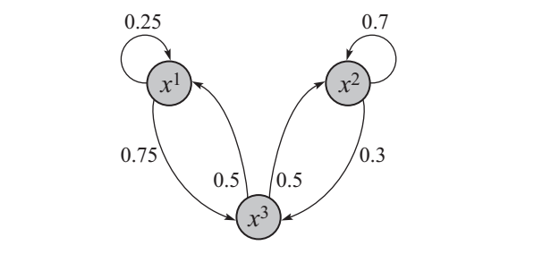 A Markov Chain for three possible values of a random variable and representing all nine transition probabilities (zero probability transitions are omitted)\(\\\)This is figure 12.4 from Koller et al. (2009).
To sample a Markov Chain means we sample an initial \(\mathbf{x}^{(0)}\in \textrm{Val}(\mathbf{X})\) according to a starting distribution \(P_\mathcal{T}^{(0)}\). Then we use the \(\mathcal{T}(\mathbf{x} \rightarrow \mathbf{x}')\) probabilities to sample the next state, producing \(\mathbf{x}^{(1)}\). This is repeated, producing a series of \(\mathbf{x}^{(t)}\)’s. If we were to restart the sampling procedure many times and select the \(t\)-th sample, we’d observe a distribution that we’ll call \(P_\mathcal{T}^{(t)}\).
Using the above Markov Chain, a sequence of samples might look as follows, where transition probabilities appear above the arrows1:
\[\xrightarrow{0.33} x^1 \xrightarrow{0.75} x^3 \xrightarrow{0.5} x^2 \xrightarrow{0.7} x^2\]By this procedure, one may infer:
\[P_\mathcal{T}^{(t+1)}(\mathbf{x}) = \sum_{\mathbf{x}' \in \textrm{Val}(\mathbf{X})} P_\mathcal{T}^{(t)}(\mathbf{x}') \mathcal{T}(\mathbf{x}'\rightarrow \mathbf{x})\]This is to say, the probability of the next state is equal to the sum of the probabilities of every other state multiplied by their respective transition probabilities.
For large \(t\) and under some technical conditions, \(P_\mathcal{T}^{(t)}\) will be similar to \(P_\mathcal{T}^{(t+1)}\). This common distribution is the stationary distribution of \(\mathcal{T}\), labeled \(\pi_\mathcal{T}\). As the single distribution that works for both \(P_\mathcal{T}^{(t)}\) abd \(P_\mathcal{T}^{(t+1)}\) in the above relation, it solves:
\[\pi_\mathcal{T}(\mathbf{x}) = \sum_{\mathbf{x}' \in \textrm{Val}(\mathbf{X})} \pi_\mathcal{T}(\mathbf{x}') \mathcal{T}(\mathbf{x}'\rightarrow \mathbf{x})\]In summary, the distribution that solves these equations, \(\pi_\mathcal{T}\), is the distribution \(P_\mathcal{T}^{(t)}\) converges to as \(t \rightarrow \infty\).
With this, we may state an essential insight:
We can choose the Markov Chain \(\mathcal{T}\) such that \(\pi_\mathcal{T} = P_M\).
Theoretically and without computational considerations, one could choose \(\mathcal{T}\) with knowledge of \(P_M\), solve the system of equations and obtain \(\pi_\mathcal{T} = P_M\). However, this is not feasible as the count of equations is equal to the count of all possible joint assignments, \(\vert \textrm{Val}(\mathbf{X}) \vert\). The point is to pave a realistic path.
To do so requires Monte Carlo methods, the second ‘MC’ in ‘MCMC’. The idea is to sequentially sample \(\mathbf{x}^{(0)}, \mathbf{x}^{(1)}, \cdots, \mathbf{x}^{(t)}\) according to a \(\mathcal{T}\) whose stationary distribution, \(\pi_\mathcal{T}\), is the distribution we seek: \(\pi_\mathcal{T} = P_M\). In other words, for large \(t\) and a properly chosen \(\mathcal{T}\), we may consider \(\mathbf{x}^{(t)}\) a sample from \(P_M\).
So, this raises a question.
How is \(\mathcal{T}\) chosen?
To select a particular MCMC algorithm is to make this choice. The algorithms’ common aim is:
to provide \(\mathcal{T}\) for which sampling will converge quickly to a single \(\pi_\mathcal{T}\), equal to \(P_M\), from any initial \(P^{(0)}_\mathcal{T}\).2
This is hard. We face the following difficulties:
-
Consider a \(\mathcal{T}\) with two states where each state always transitions to the other; there is a zero-probability of remaining in a state. This creates a strong dependence on \(P^{(0)}_\mathcal{T}\) and means a stationary distribution \(\pi_\mathcal{T}\) does not exist.
Such cyclic behavior means the Markov chain is periodic, whereby the distribution of \(\mathbf{x}^{(t)}\) depends on \(t\) modulo some time period. By analogy, no stationary distribution exists in the same way \(\lim_{t \rightarrow \infty} \sin(t)\) does not exist.
-
A \(\mathcal{T}\) with a low conductance is one in which the state space has regions for which transitions across are very unlikely. If samples are initiated in one region, it’ll take a long time before the others are explored. This creates a near-dependence on \(P^{(0)}_\mathcal{T}\). Further, convergence necessitates repeatedly traversing these low probability bridges, slowing it considerably. The following is an example of a low conductance \(\mathcal{T}\), where dotted lines indicate low transition probabilities:
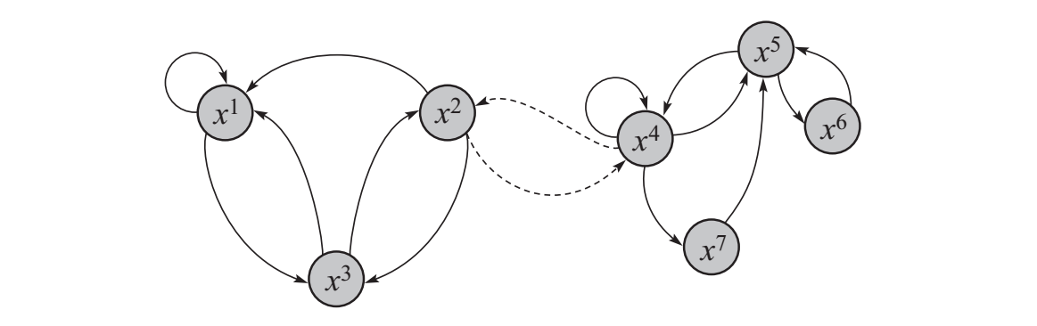 A low conductance Markov Chain\(\\\)This is figure 12.6 from Koller et al. (2009)
- \(\mathcal{T}\) is called reducible if there exists two states which cannot be reached from each other, even with infinite transitions. Consequently, there may be more than one stationary distribution.
Our protection against this unruly behavior is some theoretical properties one may demand of \(\mathcal{T}\). For example, we may guarantee it’s aperiodic.
One of the most important protections is detailed balance. A \(\mathcal{T}\) with this property obeys the following:
\[\pi_\mathcal{T}(\mathbf{x})\mathcal{T}(\mathbf{x}\rightarrow \mathbf{x}') = \pi_\mathcal{T}(\mathbf{x}')\mathcal{T}(\mathbf{x}'\rightarrow \mathbf{x})\]for any pair of \(\mathbf{x}, \mathbf{x}' \in \textrm{Val}(\mathbf{X})\).
Compare this to the previous equation of a stationary distribution, reproduced here:
\[\pi_\mathcal{T}(\mathbf{x}) = \sum_{\mathbf{x}' \in \textrm{Val}(\mathbf{X})} \pi_\mathcal{T}(\mathbf{x}') \mathcal{T}(\mathbf{x}'\rightarrow \mathbf{x})\]Its right side has many more terms, and so \(\pi_\mathcal{T}(\mathbf{x})\) suffers many more degrees of freedom. Intuitively, detailed balance implies the stationary distribution follows from single step transitions and not from cycles of many transitions. It’s a kind of well-connectedness conditioned.
All of the above can be summarized as:
If \(\mathcal{T}\) implies any two states are reachable from each other, is aperoidic and has detailed balance, then samples will converge to a unique stationary distribution from any starting distribution.
With this, we may consider our first MCMC algorithm.
Gibbs Sampling
The transitions of Gibbs Sampling involve changing each sampled vector by one element at a time. Specifically, the algorithm involves the following steps:
- Uniformly sample \(\mathbf{x}^{(0)}\) from \(\textrm{Val}(\mathbf{X})\).
- Select a variable \(X_1\) from \(\mathbf{X}\) and list \(\textrm{Val}(X_1)\). For example, \(\textrm{Val}(X_1)=[x_1^1,x_1^2,x_1^3,x_1^4]\).
- For each \(x_1^i \in \textrm{Val}(X_1)\), create a new vector by substituting \(x_1^i\) into the \(X_1\)-position of \(\mathbf{x}^{(0)}\) and label it \(\mathbf{x}^{(0)}_{i-\textrm{sub}}\).
- Plug each \(\mathbf{x}^{(0)}_{i-\textrm{sub}}\) into the Gibbs Rule3 to yield four positive numbers. Normalize them into a probability vector.
- Use the probability vector to sample one of the \(\mathbf{x}^{(0)}_{i-\textrm{sub}}\)’s and set it as \(\mathbf{x}^{(1)}\).
- Go back to step (2), but this time use \(X_2\) to produce \(\mathbf{x}^{(2)}\).
Steps (2)-(6) are repeatedly applied, cycling over the variables of \(\mathbf{X}\) many times, until we suspect samples have converged to the target distribution.
Essentially, steps (3)-(5) reflect sampling with implicitly defined transition probabilities. They are designed so that if we pick a large enough \(t\), \(\mathbf{x}^{(t)}\) will come from \(P_M(\mathbf{X})\)4 as desired.
But there’s an obvious weakness. As mentioned, \(\mathbf{x}^{(t)}\) and \(\mathbf{x}^{(t + 1)}\) will be identical except for one element and so, the sequences are strongly correlated over small differences in \(t\). In other words, such samples are not independent.
To measure the problem, we may estimate the effective sample size. This quantity enables statements of the form: “These 100 dependent samples are as good as 10 independent samples”. In this case, 10 is the effective sample size. Its utility is in measuring uncertainty, which can alert us to our samples’ infidelity. We won’t go into detail on the calculation of effective sample size, beyond mentioning it relies on measuring correlations across samples.
Further, correlation of samples isn’t the only issue; updating one variable at a time makes it slow. Fortunately, there are faster algorithms.
The Metropolis-Hastings Algorithm
We may improve beyond Gibbs Sampling if we control how fast the state space is explored. To guarantee the resulting \(\pi_\mathcal{T}\) equals \(P_M\), we’d have to apply a correction to compensate for this control. Roughly, this is the idea behind the Metropolis-Hastings algorithm.
Specifically, we invent another Markov Chain, labeled \(\mathcal{T}^Q\), which is the proposal Markov Chain. It’s defined over the same space \(\textrm{Val}(\mathbf{X})\) and is responsible for proposing the next state \(\mathbf{x}^{(t+1)}\) given the current state \(\mathbf{x}^{(t)}\). Its utility is in enabling large leaps.
The correction will be to sample an ‘accept-or-reject’ event with a specially designed acceptance probability. If an ‘accept’ is drawn, the proposal to transition to the next state is accepted. If a ‘reject’ is drawn, the proposal is rejected and a new one must be generated. The acceptance probability is:
\[\mathcal{A}(\mathbf{x}\rightarrow\mathbf{x}') = \textrm{min}\bigg(1, \frac{\widetilde{P}_M(\mathbf{x}')\mathcal{T}^Q(\mathbf{x}'\rightarrow\mathbf{x})}{\widetilde{P}_M(\mathbf{x})\mathcal{T}^Q(\mathbf{x}\rightarrow\mathbf{x}')} \bigg)\]Stated without proof, this ensures detailed balance and convergence to \(P_M\) from any starting distribution, given enough time and assuming \(\mathcal{T}^Q\) isn’t especially badly behaved.
Intuitively, \(\widetilde{P}_M(\mathbf{x}')/\widetilde{P}_M(\mathbf{x})\) makes \(\mathbf{x}'\) more likely to be rejected if \(\mathbf{x}'\) is less likely than \(\mathbf{x}\), according to \(P_M\). This is how an arbitrary \(\mathcal{T}^Q\) is corralled to produce samples of \(P_M\).
Further, \(\mathcal{T}^Q(\mathbf{x}'\rightarrow\mathbf{x})/\mathcal{T}^Q(\mathbf{x}\rightarrow\mathbf{x}')\) makes a proposed state likely to be rejected if it’s difficult to return from. In other words, transitions likely to be made but unlikely to be made in reverse are discouraged. This is what ultimately yields detailed balance.
Next, we may observe two benefits:
- Using a ratio means only unnormalized probabilities, \(\widetilde{P}_M(\mathbf{x}')\) and \(\widetilde{P}_M(\mathbf{x})\), are necessary. This avoids the need for the often intractable normalizer \(Z\).
- By design of \(\mathcal{T}^Q\), \(\widetilde{P}_M(\mathbf{x}')\) and \(\widetilde{P}_M(\mathbf{x})\) may share identical factors which cancel in the ratio. Computing these factors would be unnecessary and provides a means for saving compute.
Finally, some caution is in order:
- \(\mathcal{T}^Q\) should be able to propose everything in \(\textrm{Val}(\mathbf{X})\). Otherwise, the above properties won’t hold since the proposal may assign zero probability to something \(P_M\) ascribes positive probability to.
- A rejected proposal is a waste of compute. In this sense, we desire \(\mathcal{A}(\mathbf{x}\rightarrow\mathbf{x}')\) to be near 1 always. However, such values are unlikely to be observed with large leaps over the state space. Indeed, a value always near 1 may suggest the space isn’t being explored quickly. This tradeoff suggests \(\mathcal{T}^Q\) should be tuned such that large leaps can be made, but not so large that proposals are frequently rejected.
An Application of Metropolis-Hastings
Murphy (2012) contains an informative toy application and visualization, which we’ll discuss here. We pretend the intractable \(P_M\) is a mixture of two Guassian distributions5 producing the density:
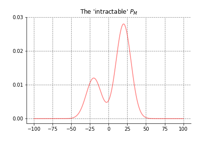
The goal is a set of samples distributed along the horizontal axis in proportion to the density. To this end, our porposal distribution will be a Gaussian centered on the current state:
\[\mathcal{T}^Q(x\rightarrow x') = \mathcal{N}(x' \vert x, v)\]where \(v\) is the variance, a term we may tune. As would be true with an actually intractable \(P_M\), we’ll assume we can compute the probability ratio \(P_M(x')/P_M(x)\). This specifies enough to generate proposals, accept or reject them and produce a set of samples. Murphy (2012) represents it with the following figure with the \(t\) dimension laid out and for three values of the tunable variance \(v\):
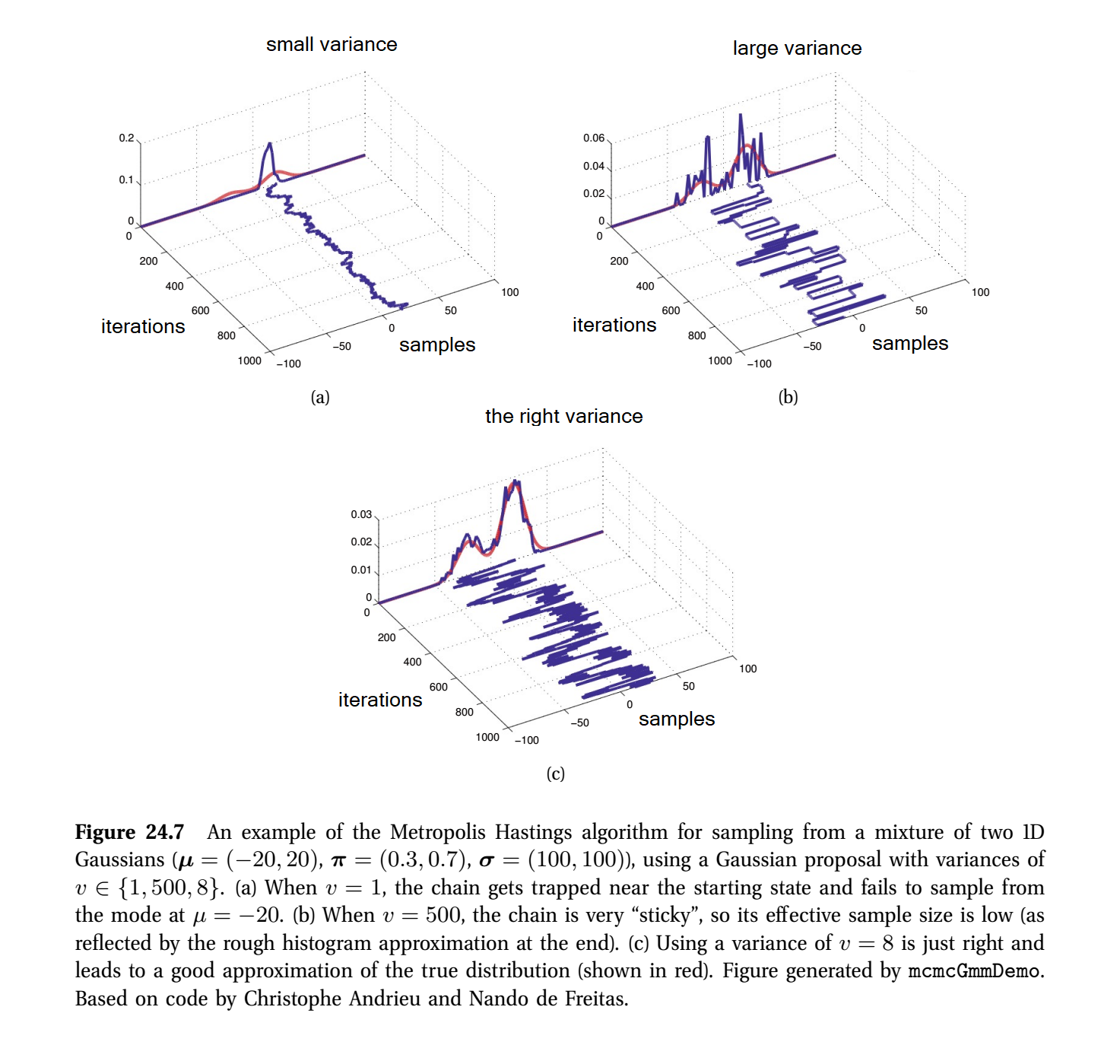 Figure 24.7 from Murphy (2012)
As is clear, tuning \(v\) defines a sweet spot where samples thoroughly explore both modes and not too many proposals are rejected. The latter point is observed with an absence of straight lines along the iterations dimension; such lines indicate proposals are repeatedly rejected.
The Next Step
Next, we consider how parameters of PGMs are learned:
References
-
D. Koller and N. Friedman. Probabilistic Graphical Models: Principles and Techniques. MIT Press. 2009.
-
K. Murphy. Machine Learning: A Probabilistic Perspective. MIT Press. 2012.
-
D. MacKay. Information Theory, Inference and Learning Algorithms. Cambridge University Press. 2003.
-
Stan contributors. Stan Reference Manual: Effective Sample Size. Stan
Something to Add?
If you see an error, egregious omission, something confusing or something worth adding, please email dj@truetheta.io with your suggestion. If it’s substantive, you’ll be credited. Thank you in advance!
Footnotes
-
The 0.33 probability comes from assuming \(P_\mathcal{T}^{(0)}\) is uniform. ↩
-
One could make the case that there is the additional aim: to provide independent samples. I’ve omitted this because a \(\mathcal{T}\) which brings fast convergence to \(P_M\) must quickly ‘forget’ the initial distribution \(P_\mathcal{T}^{(0)}\). By my intuition, this implies a reduction in sample autocorrelation; fast convergence implies more independent samples. ↩
-
There’s an efficiency to be had here. We don’t need to compute the full Gibbs Rule product; we only need to consider the factors for which \(X_1\) appears in. All factors for which \(X_1\) doesn’t appear, their product remains constant as different assignments of \(X_1\) are plugged in. Following normalization, this constant has no effect, so we need not consider it from the start. For large MNs, this creates a significant improvement in efficiency. ↩
-
\(P_M(\mathbf{X} \vert \mathbf{e})\) in fact ↩
-
Again, this is a case where we are using a continous distribution for the sake of an illustrative example. The theory, as presented, concerns only the discrete case. ↩