Part 7: Structure Learning
Posted: Updated:
This series has proceeded as:
- Inference: Given a trained PGM, how are probability queries answered?
- Parameter Learing: Given data and the graph of a PGM, how are parameters learned?
- Structure Learning1: Given data, how is the graph determined?
This is opposite the practioner’s experience. They first must accomplish (3) so they may accomplish (2) so they may perform (1)2. The series ordering follows from a dependency of concepts; inference is a prerequisite of parameter learning which, as will be shown, is a prerequisite of structure learning.
As a result, complexity increases in the order: (1), (2), (3). To learn parameters well, their consequent inferences must be anticipated. Analogously, to learn a graph well is to anticipate the parameters learned. As an example, two graphs could be compared by comparing their likelihoods achieved at the end of parameter learning3. In this case, structure learning recruits parameters learning as a subroutine and so, is more computationally intensive. This amounts to:
Essentially, structure learning involves the largest integrations of the tasks considered. In this sense, it is the hardest.
As a personal anecdote, when applying causal graphical modeling at Lyft, our team avoided algorithmic structure learning by positing and testing several candidate graphs, guided by mere intuition. The first reason was for that of causality, a quality not considered in this series. As Judea Pearl admonishes, a causal graph is an assumption not fully testable in observational data, and so domain knowledge and scarce experimental data are the determinants. The second reason was that of limited time and resources. The burden of a single graph was enough to make evaluating a sea of them out of the question. From this experience, I see two general points:
- As of 2023, current theory and opensource software can’t yet surface a reliable causal graph in practice.
- As a practical necessity, some resort to speculating the graph by domain knowledge.
Regarding the first point, our task is easier. This series isn’t concerned with causality, since the goal is to answer associative queries of a complex system, and so we may discuss structure learning as a function solely of observational data.
Regarding the second point, we should see graph speculation in historical context. Section 2.4 of Wainwright et al. (2008) describes classic applications, unaided by modern structuring learning, showing it can be done successfully. In the future, we’ll see other performant models developed without formal structure learning. Still, it is unlikely speculated graphs are optimal, and so structure learning has clear utility. Even if one doesn’t perform structure learning, understanding it informs speculation. Further, as compute and techniques improve, so will the offer of structure learning.
In this post, we’ll describe the theory of structure learning and the approximate algorithms that follow. Before proceeding, it may help to review the Notation Guide, the Part 1 summary, the Part 2 summary and either the Part 5 or the Part 6 summary.
The Starting Point and Goal of Structure Learning
Essentially but not exactly, the goal of structure learning is to learn a graph of a PGM from data. The aim is a structure that captures the CI statements of the true distribution \(P\) of a complex system of variables \(\mathcal{X}\). It needs to be done in a way such that subsequent parameter learning yields a distribution that matches empirical observations. If the model is a Bayesian Network (‘BN’), the goal is to learn its direct acyclic graph \(\mathcal{G}\). If the model is a Markov Network (‘MN’), the goal is to learn a structure akin to the undirected graph \(\mathcal{H}\) but something more specific, so as to immediately enable parameter learning with its determination.
In both cases, we assume we have data in the following form: \(\mathcal{D}=\{\mathbf{x}^{(i)}\}_{i=1}^w\) where \(\mathbf{X} = \mathcal{X}\). To start, we’ll assume \(\mathcal{D}\) is fully observed and later, we’ll discuss missing data.
To begin from this point, we consider a question.
A Bayesian Network or a Markov Network?
Upon inspecting the data, we must determine whether to use a BN or a MN. It helps to recall a comment from Part 1:
Broadly, MNs do better when we have decidedly associative observations, like pixels on a screen or concurrent sounds. BNs are better suited when the random variables represent components of some causal or sequential structure. Timestamps and domain knowledge are helpful in such a case.
From here, we assume knowledge of the system makes the choice clear.
The obvious solution that does not work
Whether we’ve decided on a BN or a MN, both imply a set of conditional independence statements. It seems clear we should use \(\mathcal{D}\) to test for such statements and select the graph which represents them. Unfortunately, this doesn’t work well for at least three reasons:
- It’s possible the set of CI statements produced is not representable with any graph.
- Since \(\mathcal{D}\) is a sample from the true distribution \(P\), we don’t expect CI statements to hold exactly in \(\mathcal{D}\). We must rely on statistical tests to determine probabilistically whether a CI statement is true. Since CI statements are strongly interrelated (one set of CI statements implies another), false conclusions propagate to create others.
- Many statistical tests are necessary, creating a strong issue of multiple hypothesis testing. In short, it is not clear how to test for sets of CI statements in a way that surfaces the most probable graph.
Since these approaches don’t work well, we consider an alternative.
Score-Based Structure Learning
The idea is to search a discrete space of graphs and to select one according to a score. To do so, we must specify the following.
Components of score-based structure learning:
- The Search Space of Structures over \(\mathcal{X}\): A point in this space corresponds to a graph or a set of graphs. The simplest space is the space of graphs themselves; a point corresponds to a set of edges4. We’ll call this the standard graph space. In contrast, an alternative (and likely useless) space is one where each point corresponds to a count of edges. In such a case, resolving to a point involves additional work, as the specific graph associated with the point’s graph set remains to be determined.
- A set of operators: Applying one defines how to move from one point in the search space to a neighboring point. For example, if we consider the standard graph space for a BN, three common operators are edge addition, edge deletion and edge reversal.
- The Score Function: This measures a point (or graph) according to some criteria. Most typically, it measures the extend to which the graph can explain the data with the use of a likelihood function.
- A Search Algorithm: Using the previous components, this determines how the space is searched to ultimately return the final point.
Components (1) and (2) are very much entangled; we cannot decide one without considering the other. Also, the score function heavily depends on the choice of search space, since it must accept a point in that space. In general, a typical score function expects a point from the standard graph space. The last component is technically agnostic of the first three, but its effectiveness isn’t. For example, if the score function is very expensive to evaluate, the best search algorithm will call that function a limited number of times.
Graph Learning of a Bayesian Network
We begin in the case of a BN. For simplicity, we’ll consider the standard graph space and select edge addition, deletion and reversal as the operators. The score function and search algorithm will be discussed in the next sections.
A natural question concerns the size of the graph space. Recalling \(n\) as the number of variables, we recognize a one-to-one correspondence between binary \(n\)-by-\(n\) matrices and directed graphs5. Such matrices are adjacency matrices and there are \(2^{n^2}\) of them and so of directed graphs. However, since we are concerned only with directed acyclic graphs (‘DAGs’), this is an overestimate. Suffice it to say the number of graphs grows like \(2^{\mathcal{O}(n^2)}\). For even a moderate \(n\), we are dealing with an astronomical space of graphs. Exhaustive search is not an option.
Desired Properties of a BN Graph Score
Before specifying a score function, we should ask what we want of it. To express it, let \(\mathcal{G}^0\) be any directed graph and \(\textrm{Score}(\cdot)\) be the score function. Implicit in this notation is the score’s dependency on the data.
Some desired properties of \(\textrm{Score}(\cdot)\) are:
-
Consistency: If we were to sample an infinite amount of data from nature’s distribution \(P\), the score function should assign its max value to the true graph.
For consistency to be obtainable, the true graph needs to be faithful to some DAG. Faithfulness means \(P\)’s CI statements can be exactly expressed as the CI statements of a DAG. Going forward, we’ll assume this to be true. More generally and as explored in Sadeghi (2017), it’s an open question whether a given \(P\) is faithful to some graph.
-
Score Equivalence: To describe this requires the concept of Markov Equivalence6. Two graphs are Markov equivalent if they imply the same set of CI statements. Perhaps surprisingly, two different graphs can imply the same CI statements7. This is important because if two graphs are equivalent, we can select their parameters such that they yield identical distributions over \(\mathcal{X}\). This is a problem since differences in likelihoods define our relative preferences across graphs. This suggests a desired property: Two Markov equivalent graphs should produce the same score, since they can explain the data equally well8.
-
Decomposable: A score for a BN graph is decomposable if it is a sum of terms, each a score of a particular family, defined as a child node plus its parents:
\[\textrm{Score}(\mathcal{G}^0) = \sum_j^n \textrm{FamScore}(X_j \vert Pa_{X_j}^{\mathcal{G}^0})\]With this, changing the graph with an operator will only impact one or two terms, greatly reducing the computations required as the search space is traversed.
In short:
We desire a score function which is cheap to update as operators are applied and will recover the Markov equivalence class of \(P\)’s graph in the limit of infinite data.
A BN Graph Score Function
To achieve the properties above, we apply Bayesian principles. We start by proposing:
\[P_B(\mathcal{G}^0 \vert \mathcal{D})\]Computing this will be burdensome and require thus far unspecified assumptions. For progress, we apply a log transform and Bayes’ theorem:
\[\begin{align} \log P_B(\mathcal{G}^0 \vert \mathcal{D}) & = \log \frac{P_B(\mathcal{D} \vert \mathcal{G}^0)P_B(\mathcal{G}^0)}{P_B(\mathcal{D})} \\ & = \underbrace{\log P_B(\mathcal{D} \vert \mathcal{G}^0) + \log P_B(\mathcal{G}^0)}_{\textrm{Score}_B(\mathcal{G}^0)} - \log P_B(\mathcal{D}) \\ \end{align}\]We see \(\log P_B(\mathcal{D})\) is constant across graphs and so, cannot discriminate them and so, does not need to be computed. What remains, labeled \(\textrm{score}_B(\mathcal{G}^0)\), will be our chosen score and referred to as the Bayesian score.
Next, we discuss assumptions, beginning with \(P_B(\mathcal{G}^0)\), the model’s probability of \(\mathcal{G}^0\) prior to observing the data. This is a new distribution to be assumed. It is an opportunity to ascribe graph probabilities by expert opinion or to apply regularization, where simpler graphs are preferred. However, with reasonably sized data and a properly weak prior, this term’s effect is minor. Here, we’ll consider it a constant.
In contrast, strong assumptions are specified with \(P_B(\mathcal{D} \vert \mathcal{G}^0)\), the probability of the data assuming knowledge only of the graph \(\mathcal{G}^0\) and for emphasis, no knowledge of specific parameters. It can be written as an integral, where familiar terms and its intractability may be recognized:
\[P_B(\mathcal{D} \vert \mathcal{G}^0) = \int_{\boldsymbol{\Theta}_{\mathcal{G}^0}} P_B(\mathcal{D} \vert \mathcal{G}^0,\boldsymbol{\theta}_{\mathcal{G}^0})P_B(\boldsymbol{\theta}_{\mathcal{G}^0} \vert \mathcal{G}^0)d \boldsymbol{\theta}_{\mathcal{G}^0}\]where:
- \(P_B(\mathcal{D} \vert \mathcal{G}^0,\boldsymbol{\theta}_{\mathcal{G}^0})\) is the likelihood according to the BN with graph \(\mathcal{G}^0\) and parameters \(\boldsymbol{\theta}_{\mathcal{G}^0}\). We’ve encountered this quantity in Part 5. Assumptions in this term include parameterization, whereby the precise functional form of parameters for computing an observation’s probability is specified.
- \(P_B(\boldsymbol{\theta}_{\mathcal{G}^0} \vert \mathcal{G}^0)\) is the prior distribution over parameters and so far has not be considered. Again, it is a new distribution to be assumed, mostly typically to serve regularization.
- \(\boldsymbol{\Theta}_{\mathcal{G}^0}\) is the space of all possible parameters. It is typically very large.
This tells us:
\(P_B(\mathcal{D} \vert \mathcal{G}^0)\) is the average of likelihoods \(P_B(\mathcal{D} \vert \mathcal{G}^0,\boldsymbol{\theta}_{\mathcal{G}^0})\) weighted by prior probabilities of their parameters \(P_B(\boldsymbol{\theta}_{\mathcal{G}^0} \vert \mathcal{G}^0)\). The integration is over an exponential large space \(\boldsymbol{\Theta}_{\mathcal{G}^0}\), making the quantity intractable in general.
To address this, the model can be designed to grant tractability at the cost of modeling capacity or approximations can be used. We will discuss the latter.
Before we do so, we state the following accomplishment:
Assuming \(\mathcal{D}\) was generated by nature’s distribution \(P\) in accordance9 with some graph \(\mathcal{G}_P\) and \(P_B(\boldsymbol{\theta}_{\mathcal{G}^0} \vert \mathcal{G}^0)\) is appropriately designed, \(\textrm{Score}_B(\mathcal{G}^0)\) is consistent, decomposable and satifies score equivalence.
Approximating the Bayesian Score
For an approximation, we have the following result for an appropriately chosen prior:
\[\begin{align} \textrm{Score}_{B}(\mathcal{G}^0) & \rightarrow \log P_B(\mathcal{D} \vert \mathcal{G}^0,\hat{\boldsymbol{\theta}}_{\mathcal{G}^0}) - \frac{\log w}{2}\textrm{Dim}(\mathcal{G}^0) + \textrm{const}\\ \textrm{as } w & \rightarrow \infty \end{align}\]where:
- \(\textrm{Dim}(\mathcal{G}^0)\) is the dimension of \(\mathcal{G}^0\). In the case of a BN, it is well approximated by \(\mathcal{G}^0\)’s count of parameters.
- \(\hat{\boldsymbol{\theta}}_{\mathcal{G}^0}\) is the MLE according to \(\mathcal{G}^0\) and \(\mathcal{D}\). It can be learned as described in Part 5.
This suggests a new score, called the Bayesian Information Criteria (‘BIC’):
\[\textrm{Score}_{BIC}(\mathcal{G}^0) = P_B(\mathcal{D} \vert \mathcal{G}^0,\hat{\boldsymbol{\theta}}_{\mathcal{G}^0}) - \frac{\log w}{2}\textrm{Dim}(\mathcal{G}^0)\]This is tractable and maintains the properties we desire; it is a reasonable choice for evaluating graphs.
A Search Algorithm over BN Graphs
All that remains to determine is a search algorithm. Assuming an initial point is provided and the components (1), (2) and (3) are specified, a simple algorithm is as follows:
- Apply the operators to the current point to produce a set of neighbors.
- Score each neighbor and set the current point to the highest scoring neighbor.
- Repeat (1) and (2) until the score stops improving by some threshold.
With the use of the standard graph space, operators of deletion, addition and reversal, and the BIC, the above specifies a valid algorithm:
It will produce a \(\hat{\mathcal{G}}\) suggested by \(\mathcal{D}\), which enables parameter learning of a model \(P_B\), which enables inference, which enables insight into nature’s distribution \(P\) of a complex system \(\mathcal{X}\).
This is not to trivialize the task, but to reveal a walkable path. In practice, we anticipate at least the following challenges:
- The algorithm is likely to face local optima.
- If an operation yields a neighbor within the same Markov equivalence class as the current point, the score will be and should be the same. In this case, it’s a waste to compute the neighboring score. Ideally, operations should always traverse equivalence classes, but this is not easy to design.
This is to suggest we’re floating above miles of depth. See chapter 3 of Y. Zhou (2011) for an in-depth review of the topic. Here, we’ll move onto the next type of PGM.
Markov Network Structure Learning is Hard in General
As was discussed in Part 6, this problem is significantly harder with Markov Networks. Since roadmapping MN structure learning in general is well beyond our scope, we will instead discuss what makes it difficult using a specific MN form. As was discussed in Part 6, this problem is significantly harder with Markov Networks. Since roadmapping MN structure learning in general is well beyond our scope, we will instead discuss what makes it difficult using a specific MN form.
First, we’ll consider the log-linear form as introduced previously:
\[P_M(X_1,\cdots,X_n) = \frac{1}{Z} \exp\big(\sum_{j = 1}^m \theta_j f_j(\mathbf{D}_j)\big)\]where \(Z\) is the normalizer, assuring probabilities integrate to one over all assignments. Unlike in Part 6, we no longer constrain the \(f_j(\mathbf{D}_j)\)’s to be indicator functions; they may be any function mapping assignments to numbers.
Next, there exists an ambiguity to be addressed:
In general, knowing the MN graph \(\mathcal{H}\) is not enough to know \(m\) and the sets of variables \(\{\mathbf{D}_j\}_{j=1}^m\).
To see this, we consider a factor graph, a graph whereby factors are represented as square nodes and their respective variables are connected circular nodes. It is the factor graphs which specify the necessary information to know the scope, the \(\mathbf{D}_j\)’s, of each \(f_j(\mathbf{D}_j)\). Figure 4.8 from Koller et al. (2009) makes this ambiguity clear, where factors are denoted with \(V\):
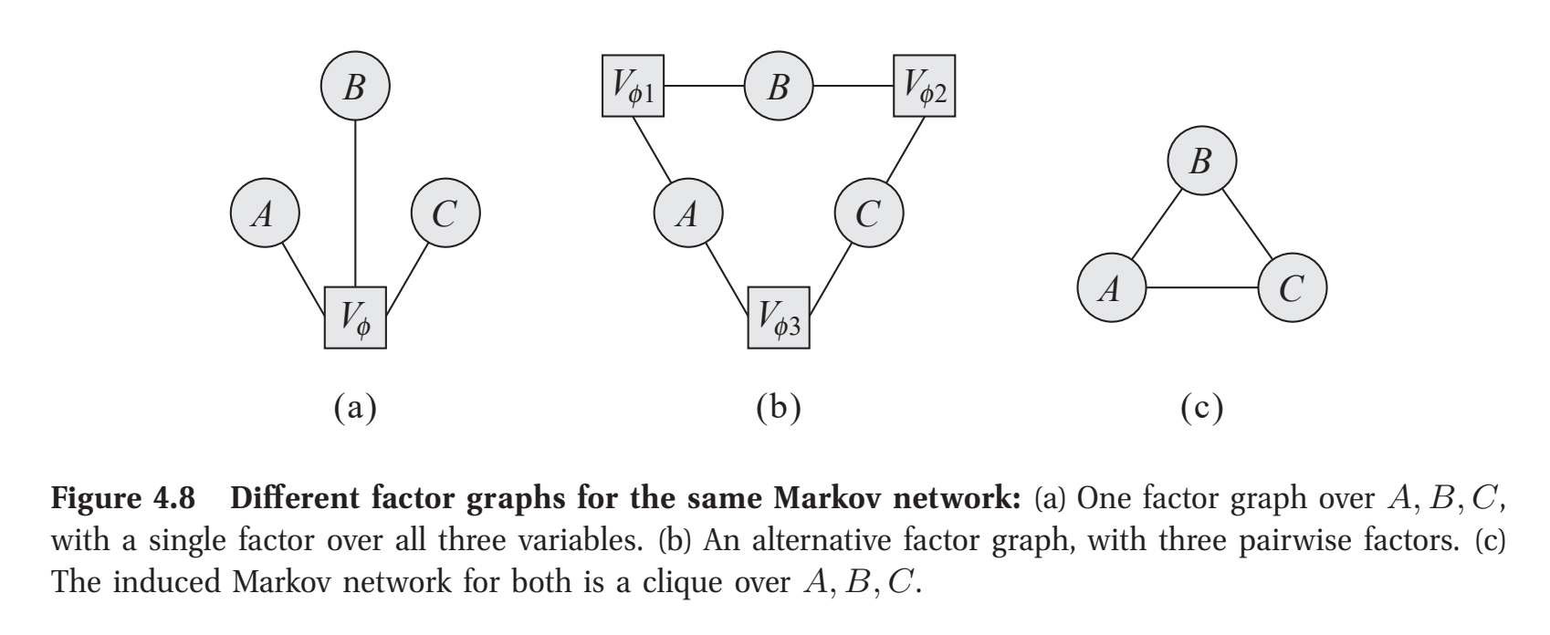 figure 4.8 from Koller et al. (2009)
This suggests learning \(\mathcal{H}\) is insufficient to begin parameter learning. Further, even if the \(\mathbf{D}_j\)’s were known, the \(f_j(\mathbf{D}_j)\)’s–the specific mappings of assignments to numbers–remain unresolved. Here, we prefer structuring learning whose completion immediately permits parameter learning. To this end, we will consider the same score-and-search components as earlier.
Score Based Structure Learning for a Markov Network
For component (1), we must suppose a space, no longer accurately described as a space of graphs, whereby a point fixes \(\{f_j(\mathbf{D}_j)\}_{j=1}^m\). For emphasis, a point must imply a choice of \(m\), a choice of scopes \(\{\mathbf{D}_j\}_{j=1}^m\) and a choice of functions mapping assignments to numbers \(\{f_j(\cdot)\}_{j=1}^m\).
This presents a large range of possibilities. It could be designed such that:
- A point corresponds to some measure (e.g. treewidth) of the complexity of the implied \(\mathcal{H}\), which has implications for the efficiency of inference and statistical properties of parameter learning. By the same reasoning, we note spaces without such a connection suffer complicated relationships with the \(\mathcal{H}\)’s, making them difficult to manage.
- Operations enumerating and scoring neighbors are computionally efficient.
- Steps to neighbors represent large leaps in model space, so a larger space of models may be explored.
As an example, we discuss the space described as follows. Consider \(\Omega\), the set of indicator functions, one for every joint assignment of every subset of \(\mathcal{X}\). Its size \(\vert \Omega \vert\) is exponentially large. A point, labeled \(\mathcal{F}^0\), corresponds to a subset of \(\Omega\), whereby indicators are selected as features of \(P_M\). The space of all points corresponds to the powerset of \(\Omega\). There are \(2^{\vert \Omega \vert}\) points in this space, so there is no possibility of exhaustive search.
The operations will be addition and deletion of indicators. Let \(\vert \mathcal{F}^0 \vert\) be the count of selected indicators. Addition corresponds to adding one of the \(\vert \Omega \vert - \vert \mathcal{F}^0 \vert\) indicators not in \(\mathcal{F}^0\) and deletion corresponds to deleting one indicator of \(\mathcal{F}^0\). Note that since \(\vert \Omega \vert\) is large, enumerating all neighbors is likely not possible.
For reasons similar to those from earlier, we’ll use the BIC score:
\[\textrm{Score}_{BIC}(\mathcal{F}^0) = P_M(\mathcal{D} \vert \mathcal{F}^0,\hat{\boldsymbol{\theta}}_{\mathcal{F}^0}) - \frac{\log w}{2}\textrm{Dim}(\mathcal{F}^0)\]Upon inspection, we see a problem. It involves computing \(\hat{\boldsymbol{\theta}}_{\mathcal{F}^0}\), which we discovered, in Part 6, is hard in general. But in this context, the problem is multiplied by the need to perform this operation for consideration of every neighbor10.
Further, this score is no longer decomposable; the score difference between neighboring points no longer amounts to a single term. In the naive construction presented, the score needs to be entirely recomputed for each of an exponential count of neighbors.
Suffice it to say, Markov Network structure learning does not enjoy the same computational advantages as that of Bayesian Networks.
Regarding Missing Data
For reasons mentioned in Part 5 and Part 6, missing data makes everything harder. It complicates computing the likelihood by necessitating an integration over missing values, which is a subroutine of structuring learning nested several levels down. Any inflation of its compute expands the demands of every section, at least as presented here. Such issues make imputation or dropping observations tempting.
Other Techniques, Briefly
The above fails to represent the diversity of techniques available. We briefly describe a few of them:
-
Assume the graph is a tree: For an undirected graph, a tree is one in which there is exactly one path between any two nodes. For a directed graph, a tree, technically a polytree, is one in which making all edges undirected yields an undirected tree. In both cases, this greatly eases structure learning and the subsequent inference. For instance, we can use the Chow-Liu algorithm to efficiently find the maximum likelihood tree. See section 26.3.2 of Murphy (2012) for a description.
-
Assume linearity and the Gaussian distribution: Despite this series’ focus on the discrete case, these continuous case assumptions are so powerful as to be worth mentioning. All variables are assumed to be real valued.
For a BN, assume all CPDs are those of linear regression; variables are normally distributed with means constructed as linear combinations of their parents. This makes all variables distributed as a single multivariate normal, whereby there is a closed form expression for the parameters’ marginal likelihood. This greatly enhances the above score based approach. In fact, this also yields closed formed expressions for the subsequent inference tasks.
For a MN, there is only the Gaussian assumption. This again induces all variables to be distributed as a multivariate normal, albeit one of a different form than in the BN case. In fact, any multivariate normal can be represented as a pairwise MN, whereby no factor involves more than two variables. By this light, the assumption is a constraint on factors’ scopes. To avoid the details (which are in section 27.2 of Murphy (2012)), this simplification enables structure learning and parameter learning in the form of an optimization of a tractable convex objective function, something akin to the lasso objective, and so it’s named the graphical lasso (‘glasso’).
-
For missing data, the Cheeseman-Stutz approximation can be applied in the BN case and variational techniques can be applied in both the MN and BN case.
Bayesian Model Averaging
We’ve so far suggested a discrete choice of structure. A set of structures, whether they be a BN graph \(\mathcal{G}\) or a selection of features, are searched and evaluated to produce a single structure, from which parameter learning may take place. This follows from the convenience of only having to subsequently perform parameter learning once and the assumption that nature’s distribution adheres to one structure.
But this latter point is unlikely to hold; most complex systems don’t in fact correspond to one structure. They are approximations made under constraints of limited observations and computation.
Inevitably, we face uncertainty about the structure. As the Bayesian philosphy recommendations, our uncertainty should be represented as a distribution. This is the idea behind Bayesian Modeling Averaging. Briefly, it suggests no discrete choice should be made. Rather, we should average probabilities across structures with weights as each structure’s probability, conditional on the data. This multiplies the computational burden, but avoids the errors of discrete structure choice.
Omissions and Caveats
This series toured the essentials of Probabilistic Graphical Models. It is no attempt at a comprehensive view; it’s a speedy walk through the terrain to expose the foundation, point the depth in every direction and prove it’s traversable on two feet. But this shouldn’t fool us into underestimating the challenge of a complex system. A few things to emphasize:
- We have not considered causality. The question of how a system will respond to an intervention necessitates more theory and creates some futility in observational data.
- We have assumed the complex system is governed by a fixed joint probability distribution \(P\). In reality, this may not even be a useful approximation, as can be the case with non-stationary systems.
- We have assumed the set of variables \(\mathcal{X}\) is given, fixed, discrete and at least partially observed. The choice of what to measure is a challenge all its own (see the grounding problem) and we’ve eschewed the design of hidden variables, which can greatly reduce parameter counts (see section 26.5.3 of Murphy (2012)).
- We have avoided questions of model parameterization. Crafting the functional form of a CPD or a factor to best capture reality while presenting an estimatable set of parameters is an essential art we haven’t covered.
- We have made no recommendation of software, yet. The first step of an application is to install software that enables this type of modeling. No advice has been provided here because the proper choice will be problem specific and as of 2023, there doesn’t appear to be widely available, up-to-date and well supported software that implements these concepts in the form presented here.
Regarding Software
The last bullet raises a question:
If PGMs are so useful, why isn’t there widely available, up-to-date and well supported software to implement them?
It’s something I’ve wondered. The answer I speculate is there is software, but no single package does the whole of probabilistical graphical modeling. The generalized endeavor is just too large. Instead, there’s software that enables subsetting or overlapping cousins of PGMs. Here is a list as of September 2023 I’d comfortably rely on:
- Stan, Pymc and Pyro are implementations of probabilistic programming, which, as described in Ghahramani (2015), is a generalization of probabilistic graphical modeling. Here, the graphical model is replaced with a more general program. With a special emphasis on Bayesian principles, the approach is the same. A program is used to specify assumptions (possibly representable as a graph) and a data generating process. Data is provided, conditioned on and a posterior over variables is produced, either via MCMC or variational methods. Notably, as is the Bayesian virtue, parameters \(\boldsymbol {\theta}\) and variables \(\mathcal{X}\) can be treated identically, collapsing the tasks of inference and parameter learning into one.
- Dynamax implements a full suite of algorithms on state-space models, a subclass of PGMs with variables indexed by time. See chapter 29 of Murphy (2023) for a comprehensive review of the topic. Notably, the author is a developer of Dynamax.
- PyTorch, Jax and TensorFlow are arguably PGM implementations and certainly useful for modeling complex systems. They implement neural networks, a hierarchical flavor of graphical models and come with distributional capacities (e.g. TensorFlow Probability). Together, they enable a type of probabilistic graphical modeling, where graphs are easily expressed, automatic differentiation eases gradient based optimization and variables aren’t treated probabilistically by default but can be. On the other hand, generalized inference is not offered; these tools don’t provide means for computing posteriors given observations of arbitrary variable. That requires extensions (e.g. Pyro is built on PyTorch).
References
-
D. Koller and N. Friedman. Probabilistic Graphical Models: Principles and Techniques. MIT Press. 2009.
-
K. Murphy. Machine Learning: A Probabilistic Perspective. MIT Press. 2012.
-
M. J. Choi, V. Y. F. Tan, A. Anandkumar and A. Willsky. Learning Latent Tree Graphical Models. Journal of Machine Learning Research. 2011.
-
Y. He, J. Jia and B. Yun. Counting and Exploring Sizes of Markov Equivalence Classes of Directed Acyclic Graphs. Journal of Machine Learning Research. 2015.
-
K. Sadeghi. Faithfulness of Probability Distributions and Graphs. Journal of Machine Learning Research. 2017.
-
Y. Zhou. Structure Learning of Probabilistic Graphical Models: A Comprehensive Survey. Arxiv. 2011.
-
Z. Ghahramani. Probabilistic Machine Learning and Artificial Intelligence. Nature volume 521. 2015
-
K. Murphy. Probabilistic Machine Learning: Advanced Topics. MIT Press. 2023.
Something to Add?
If you see an error, egregious omission, something confusing or something worth adding, please email dj@truetheta.io with your suggestion. If it’s substantive, you’ll be credited. Thank you in advance!
Footnotes
-
We call it structure learning rather than graph learning because the latter isn’t properly general. As will be seen with Markov Networks, it’s not necessarily the graph that is learned. ↩
-
To clarify, this separation of tasks exists only in principle. In practice, decisions for (1), (2) and (3) needs to be considered together. Approximations made at one level will impact operations at another, so one cannot consider them independently. In fact, some approaches straddle them intentionally and sell themselves as an attractive management of cross task tradeoffs. ↩
-
This approach, evaluating graphs by their likelihood of their respective MLEs, is not recommended. As graphs increase in edge count, their maximum achievable likelihood increases. This means the approach will select for the most complicated and overfit graphs. ↩
-
It does not correspond to a set of nodes. We assume all graphs are over the variables \(\mathcal{X}\). We are not considering searching over the space of hidden variables, which is infinite. However, see M. Choi (2011) for how it can be done, granted some assumptions are made about the latent structure. ↩
-
Specifically, this matrix has a one at row \(i\) and column \(j\) if the graph has the edge \(X_i \rightarrow X_j\). ↩
-
A detailed discussion of the relationship of DAGs and their Markov equivalence classes can be found in Y. He, (2015). ↩
-
It is known that two directed graphs are Markov equivalent if they have the same skeleton and v-structures. The skeleton of a directed graph is the undirected graph created by converting all edges to undirected edges. A v-structure is where we have three nodes \(A\), \(B\) and \(C\) where \(A\rightarrow B \leftarrow C\). To put it simply, v-structures are the only orientation of edges that make a difference for the CI statements, so they must be tracked. ↩
-
This can be seen as applying the principle of insufficient reason. ↩
-
‘In accordance’ means \(\mathcal{G}_P\) is a perfect map of \(P\), meaning \(\mathcal{G}_P\)’s CI statements equals \(P\)’s CI statements. ↩
-
This omits some computational shortcuts, like those which leverage our construction’s parallel to L1 feature selection. ↩