Bayesian Optimization
Posted: Updated:
The goal of Bayesian optimization is to find an approximate minimum to an expensive function \(f(\mathbf{x})\). This function accepts a vector \(\mathbf{x}\in\mathbb{R}^D\), returns a value, provides no gradient information and takes a long time doing it.
Despite the task’s ostensible futility, Bayesian optimization manages an effective approach. It exploits the assumed smoothness of \(f(\mathbf{x})\) to guide a search more effective than the standard alternative, random search. For illustration:
An Example
Suppose we’d like to find the minimum of this one dimensional function:
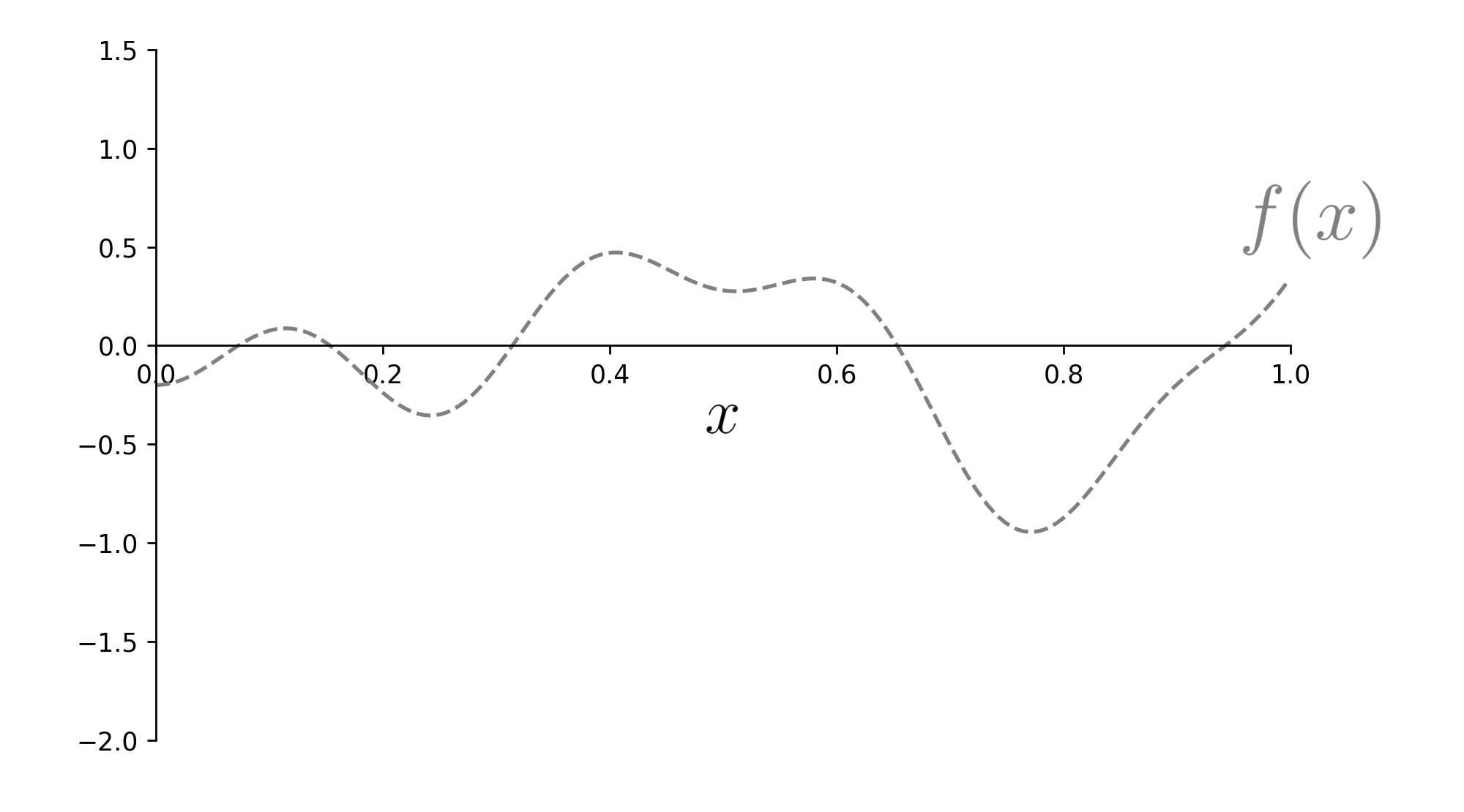 The goal is the find the function’s minimum, given a limited budget of function calls.
The dotted lines are to suggest we can’t see \(f(x)\); we may only evaluate it at selected points.
Since the function is costly, we say we have a fixed budget of evaluations; we may only evaluate it, say, ten times1. With that, how should we find the lowest minimum? One naive idea is as follows.
Random Sampling
Randomly select ten points to evaluate and take the minimum:
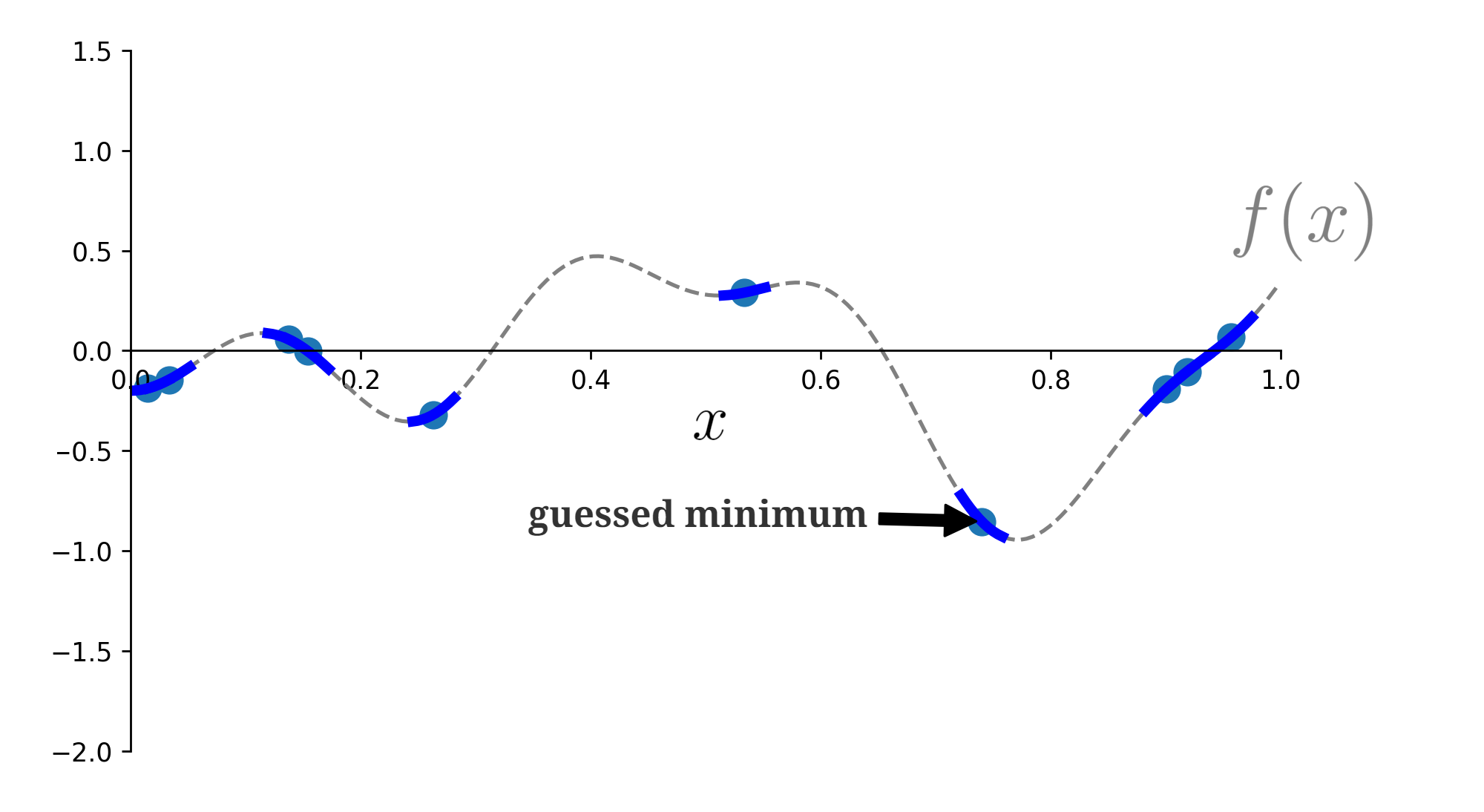 \(f(x)\) is evaluated on ten randomly sampled points.
Given enough points, this will work. But with Bayesian principles, we can do better.
Bayesian Optimization with Gaussian Processes
The idea:
Sample a number of randomly determined \((\mathbf{x}_i, f(\mathbf{x}_i))\) pairs less than the function call budget and record the minimum. Using a Gaussian process (‘GP’), infer a distribution over \(f(x)\) to inform the next points to evaluate. Once evaluated, update the running minimum if necessary and update the GP with the new observations. Repeat this until the budget is exhausted.
If the GP is any good at inferring the likely positions of \(f(x)\), this approach will outperform random sampling.
GPs are a deep topic, but for our purposes, we only need one fact. Given a dataset of input-outputs, a GP allows one to infer a distribution of likely values of \(f(x_0)\) for any given \(x_0\). For example, it enables statements like ‘There is a 0.7 probability \(f(.4)\) is between -0.5 and 0.25’. To make this clear, after sampling four points, the GP provides the information colored green:
 A GP provides distributional information over likely values of \(f(x)\) when given four \((x, f(x))\) pairs. \(\\\) According to this data, the expected value of \(f(x)\) at \(x\) is \(\mu(x)\).
Above, the green line is the GP’s guess of the true function. Each band of green is a half standard deviation of the distribution over \(f(x)\).
The Acquisition Function
At this point, we face a question: Given the GP, how do we determine the next points to evaluate? Before answering this, we’ll describe what’s desirable qualitatively.
- Since we seek the minimum of \(f(x)\), we should select points expected to produce low values.
- We should select points in regions where we’re highly uncertainty, since those regions may contain low values of \(f(x)\).
Balancing (1) and (2) is an example of the notoriously difficult exploration-exploitation trade-off. That is, we must weigh optimizing the function as it’s currently understood against improving our understanding. Fortunately, striking the perfect balance isn’t necessary to beat random sampling. To this end, we use the following:
We express our preferences for choosing the new points with an easy-to-search acquisition function, \(A(x)\). Points that yield high values of \(A(x)\) are selected as points to be evaluated.
There is a variety of acqusition functions to choose from; we’ll discuss one called expectation of improvement, \(A_{\textrm{EI}}(x)\). It gives the expected difference between the current running minimum \(\hat{x}\) and \(x\). It is computed as:
\[A_{\textrm{EI}}(x) = \sigma(x)\big(\gamma(x)\Phi(\gamma(x)) + \mathcal{N}(\gamma(x))\big)\]where:
- \(\mu(x)\) is the expected value of \(f(x)\) at \(x\).
- \(\sigma(x)\) is the standard deviation over \(f(x)\) at \(x\). It is proportional to the green width seen above.
- \(\gamma(x) = (f(\hat{x}) - \mu(x)) / \sigma(x)\) is a z-score relate to the current lowest value \(f(\hat{x})\).
- \(\Phi(\cdot)\) and \(\mathcal{N}(\cdot)\) are the CDF and PDF of the standard normal distribution, respectively.
This quantifies the appeal of all points over the search space. Naturally, we optimize it to determine the next points. Visually, this amounts to:
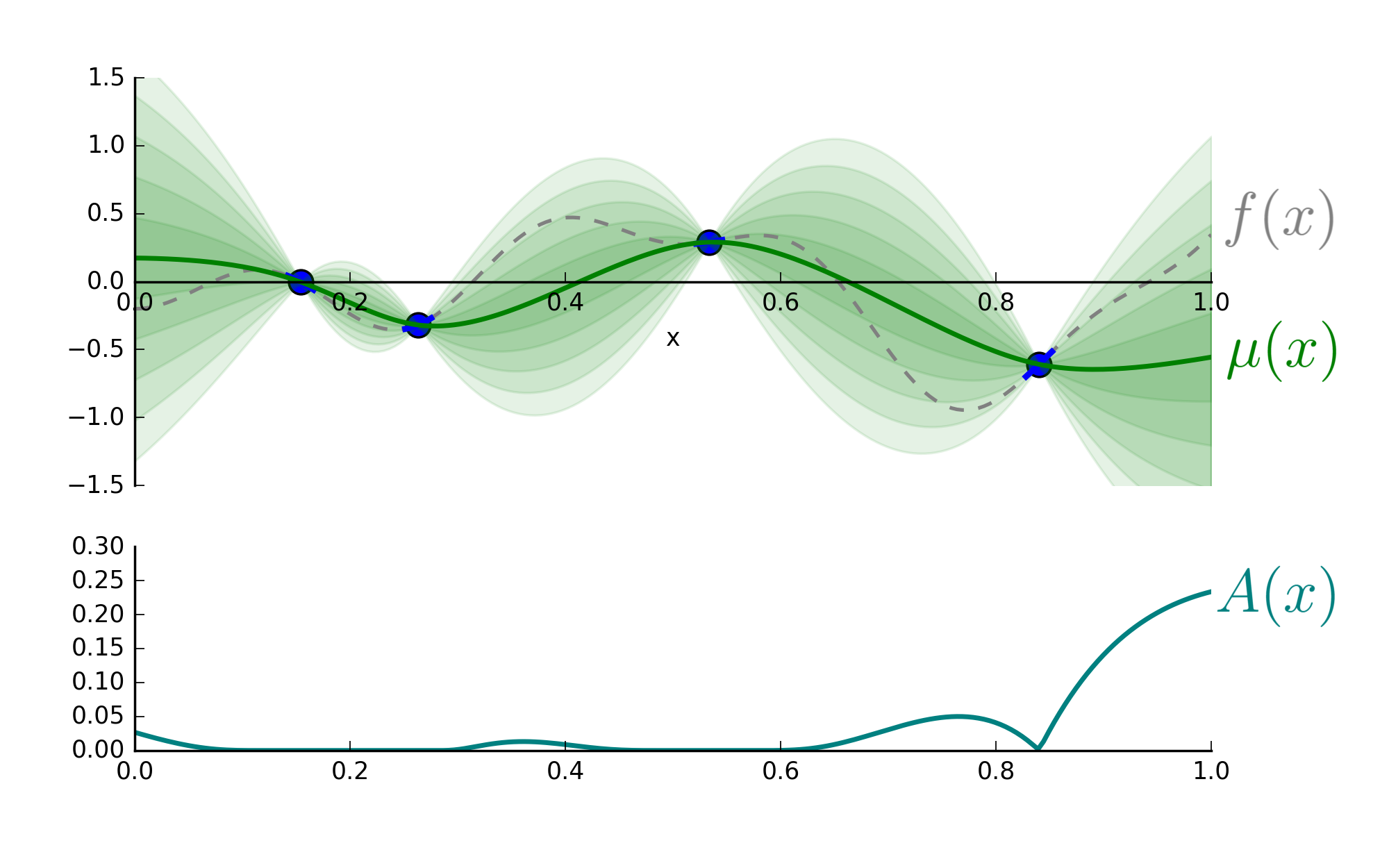 High values of the acquisition function, \(A(x)\), indicate points to evaluate next.
The above suggests the fifth point to evaluate is \(x=1\). It wouldn’t yield a new minimum, but it would substantially reduce uncertainty about \(f(x)\).
Final Comments
We’ve seen the core concept of Bayesian optimization. By using a GP to infer the likely shape of \(f(x)\), it can outperform random sampling by more prudently selecting points, ones determined with a consideration for minimizing \(f(x)\) and reducing uncertainty.
But like all toy examples, this only partially represents reality. To reduce the gap, we make the following comments:
- Generally, \(\mathbf{x}\) is a vector, not a one dimensional value. GPs scale to vectors naturally, but their effectiveness breaks down in high dimensions.
- The above suggests there is no noise in the evaluation; we observe precisely the true \(f(x)\) rather than a corrupted version \(f(x) + \epsilon\). This can be relaxed when constructing the GP.
- Designing the GP for effective inference is a skill. For a brief tutorial, consider viewing my video on the subject. Further, Duvenaud (2014) provides a more in depth view, especially on the design of kernels. For the ambitious reader, Rasmussen et al. (2006) provides a rigorous and comprehensive review of GPs.
- In a broader context, random sampling or quasi-random sampling may be preferable to Bayesian optimization. For instance, Godbole et al. (2023) point out reproducibility and statistical inference are easier when points aren’t sampled adaptively.
References
J. Snoek et al. (2012) was the primary source for this post. Rasmussen et al. (2006) provides a principled and comprehensive review of Gaussian processes in general.
-
J. Snoek, H. Larochelle and R. Adams. Practical Bayesian Optimization of Machine Learning Algorithms. Advances in Neural Information Processing Systems 2012
-
C. E. Rasmussen and C. K. I. Williams. Gaussian Processes for Machine Learning. MIT Press. 2006.
-
V. Godbole, G. E. Dahl, J. Gilmer, C. J. Shallue and Z. Nad. Deep Learning Tuning Playbook. 2023.
-
D. Duvenaud. Automatic Model Construction with Gaussian Processes. University of Cambridge. 2014.
Something to Add?
If you see an error, egregious omission, something confusing or something worth adding, please email dj@truetheta.io with your suggestion. If it’s substantive, you’ll be credited. Thank you in advance!
Footnotes
-
If you’ve tuned a machine learning model overnight, a budget of function calls should feel fitting. ↩