Part 2: Exact Inference
Posted: Updated:
We begin with a definition:
Inference: The task of answering queries of a fitted PGM.
This amounts to computations on the model. Exact inference algorithms perform these computations exactly. They primarily exploit two mechanism for efficiency:
- Factorization: The algorithms perform query transformations akin to \(ac + ad + bc + bd \rightarrow (a+b)(c+d)\), essentially seeking to multiply wherever possible, reducing the number of operations.
- Caching: A query is likely to involve redundant operations. Cleverly storing outputs enables trading memory for shortcutting computation.
Before proceeding, it may help to review the Notation Guide and the Part 1 summary.
The Gibbs Table
In our efforts to understand inference on a fitted PGM, it’ll help to imagine the ‘Gibbs Table.’ It lists all joint assignments of \(\mathcal{X}\) and the product of factors associated with each.
Consider an example; suppose we have the system \(\mathcal{X}=\{C,D,I,G,S\}\) where each random variable can take one of two values. Further, assume we have the factors determined:
\[\begin{align} &\phi_1(C) \\ &\phi_2(C,D) \\ &\phi_3(I) \\ &\phi_4(G,I,D) \\ &\phi_5(S,I) \\ \end{align}\]By ‘factors determined,’ we mean the factors have been fit to the data and are known. An example of such information is:
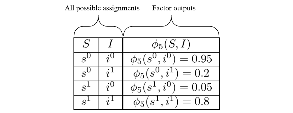 An example of a known factor
With this, the Gibbs Table looks like:
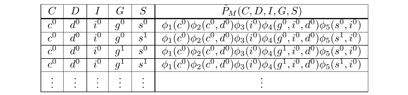 The Gibbs Table
Since the factors are known, the rightmost column, the unnormalized probabilities, have known numeric values. We express them symbolically because it aids the explanation.
As an aside, it’s worth calling out that due to the overlap between Bayesian Networks and Markov Networks mentioned previously, we may think of Bayesian Networks as representable with a Gibbs Table. As such, all discussion of the table applies to both model categories.
In general, this table is exponentially large, and so we want to think about it, but never actually write it down.
Conditioning means Filtering the Gibbs Table
With this view, consider the probability query \(P_M(\mathbf{Y} \vert \mathbf{e})\). Bayes’ Theorem tells us:
\[P_M(\mathbf{Y} \vert \mathbf{e})=\frac{P_M(\mathbf{Y},\mathbf{e})}{P_M(\mathbf{e})}\]Both the numerator and the denominator concern rows of the Gibbs Table where \(\mathbf{E}=\mathbf{e}\). The denominator is the sum of all such rows and the numerator refers to a partitioning of these rows into groups where any two rows are in the same group if they have the same assignments to \(\mathbf{Y}\). If this isn’t clear, it’ll be made so shortly.
But first, note that the act of conditioning on \(\mathbf{E}=\mathbf{e}\) makes all rows that don’t agree with the observation irrelevant; those rows can be discarded. Said differently, all times we deal with a factor that involves \(\mathbf{E}\), we plug in the \(\mathbf{e}\)-values, meaning factor outputs for non-\(\mathbf{e}\)-values have no impact on the query.
Consequently, we may define a new MN with \(\mathbf{E}=\mathbf{e}\) fixed. This is called reducing the Markov Network. The result is a new graph, labeled \(\mathcal{H}_{ \vert \mathbf{e}}\), where we delete the \(\mathbf{E}\) nodes and any edges that involve them. Also, we get a new set of factors, labeled \(\Phi_{ \vert \mathbf{e}}\), which are the original factors, but with the \(\mathbf{e}\)-values fixed as inputs. The normalizer in this reduced network, \(Z_{ \vert \mathbf{e}}\), is just \(P_M(\mathbf{e})\).
In summary:
Conditioning is equivalent to filtering the Gibbs Table on \(\mathbf{E}=\mathbf{e}\). The resulting rows define a reduced Markov Network.
To solidify intuitions, we consider the following example.
An Example: Naively Calculating \(P_M(\mathbf{Y} \vert \mathbf{e})\)
Suppose \(\mathbf{Y}=\{D,I\}\) and \(\mathbf{E}=\{G\}\). The probability query is:
What is the distribution of \(\{D,I\}\) given we observe \(G=g^0\)?
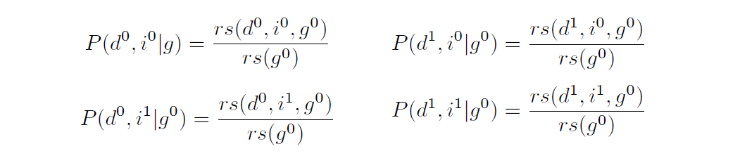
That is, we want to calculate \(P_M(D,I \vert g^0)\). To begin, consider only the probability \(P_M(d^0, i^1 \vert g^0)\), one of several asked for with \(P_M(D,I \vert g^0)\).
Following the previous argument, we start by filtering the table to rows where \(G=g^0\). Summing these rows will yield the Bayes’ Theorem denominator \(P_M(g^0)\). Of these rows, summing those where \(D=d^0\) and \(I=i^1\) will yield the numerator \(P_M(d^0, i^1, g^0)\), giving all we need to calculate \(P_M(d^0, i^1 \vert g^0)\).
From this, we see:
The core process is filtering to rows in agreement with some assignment and summing their unnormalized probabilities. We’ll refer to this as the row sum function \(rs(\cdots)\).
Specifically, \(rs(d^0, i^1, g^0)\) gives us the numerator and \(rs(g^0)\) gives us the denominator. That is, we calculate:
\[P_M(d^0,i^1 \vert g^0) = \frac{rs(d^0,i^1, g^0)}{rs(g^0)}\]Next, we consider a problem; such summations could be over a prohibitively large number of rows. To this end, we have the following.
A Simple Compute Saver
Ultimately, we care about probabilities for all assignments of \(D\) and \(I\), not just \(D=d^0\) and \(I=i^1\). That is, we want to calculate these four probabilities:
The four joint assignments of \(D\) and \(I\) partition the \(g^0\)-rows into four groups. Therefore, the numerators sum to the denominator, which is the same for all four probabilities. That is:
\[rs(g^0) = \sum_D \sum_I rs(D,I, g^0)\]This means we never need to calculate \(rs(g^0)\) directly; we need only calculate the numerators first and sum them at the end to get the denominator.
Factoring
We’ve reduced the problem to computing \(rs(\cdots)\) efficiently. As an example, consider the rows of \(rs(c^1)\):
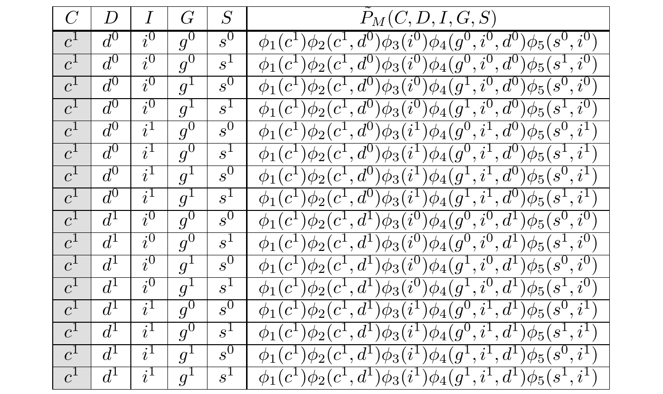 The Gibbs Tables filtered to \(C = c^1\)
If we count the operations, we see we have 4 multiplications per row and 15 summations, giving us \(4 \times 16 + 15 = 79\) operations. In the non-toy case, this number would be exponentially larger. However, we can already see opportunities for saving compute.
First, notice we are multiplying \(\phi_1(c^1)\) in every row. If it were factored out, we’d save 15 operations.
Second, consider summing the first two rows with \(\phi_1(c^1)\) pulled out:
\[\small \phi_2(c^1,d^0)\phi_3(i^0)\phi_4(g^0,i^0,d^0)\phi_5(s^0,i^0) + \phi_2(c^1,d^0)\phi_3(i^0)\phi_4(g^0,i^0,d^0)\phi_5(s^1,i^0)\]This involves 7 operations (6 multiplications and 1 sum). However, upon inspection, we see that only \(\phi_5(\cdots)\) changes across the left and right term. Again, this is an opportunity to factor:
\[\phi_2(c^1,d^0)\phi_3(i^0)\phi_4(g^0,i^0,d^0)\big(\phi_5(s^0,i^1) + \phi_5(s^1,i^1)\big)\]This reduces the count of operations to 4. So we see:
Factoring sums of products into products of sums saves compute.
As the table gets large, so will the savings.
Caching
Again, consider summing the first two rows from the Gibbs Table:
\[\small \phi_2(c^1,d^0)\phi_3(i^0)\phi_4(g^0,i^0,d^0)\phi_5(s^0,i^0) + \phi_2(c^1,d^0)\phi_3(i^0)\phi_4(g^0,i^0,d^0)\phi_5(s^1,i^0)\]The calculation of the left term involves the following operations:
\[\begin{align} v_1 \leftarrow \, & \phi_2(c^1,d^0)\phi_3(i^0) \\ v_2 \leftarrow \, & v_1\phi_4(g^0,i^0,d^0) \\ v_3 \leftarrow \, & v_2\phi_5(s^0,i^0) \end{align}\]The \(v\)’s are intermediate values as the computation is performed and \(v_3\) is the left term.
Next, consider something similar for the right term:
\[\begin{align} w_1 \leftarrow \, & \phi_2(c^1,d^0)\phi_3(i^0) \\ w_2 \leftarrow \, & w_1\phi_4(g^0,i^0,d^0) \\ w_3 \leftarrow \, & w_2\phi_5(s^1,i^0) \end{align}\]Notice we’ve performed redundant computations since \(v_1 = w_1\) and \(v_2 = w_2\). If we had cached \(v_2\), then upon computing the right term, we’d only need to perform the last line of computation.
In summary:
Inference involves redundant computations, so caching past computations enables skipping future ones.
Factoring and caching sit at the foundation of exact inference algorithms. At this point, we’re prepared to discuss one.
The Variable Elimination (‘VE’) Algorithm
There’s a single factoring technique that enables the Variable Elimination algorithm. We begin by stating it semi-generally. Suppose we are to compute \(rs(\mathbf{x})\), corresponding to an assignment for some \(\mathbf{X} \subset \mathcal{X}\). Suppose \(\mathbf{Z} = \mathcal{X} - \mathbf{X}\) and \(Z_0 \in \mathbf{Z}\) is a selected variable1. Further, suppose there are only two factors, \(\phi_1(\mathbf{D}_1)\) and \(\phi_2(\mathbf{D}_2)\), where \(\mathbf{D}_1 \cup \mathbf{D}_2 = \mathcal{X}\), and \(Z_0\) is not in \(\mathbf{D}_2\). In this case, we are to compute:
\[rs(\mathbf{x}) = \sum_{\mathbf{Z}} \phi_1(\mathbf{D}_1) \phi_2(\mathbf{D}_2)\]Implicit in the notation, if an \(X_j\) from \(\mathbf{X}\) is in one of the \(\mathbf{D}_i\) sets, then it takes on the \(x_j\) assignment in \(\phi_i(\mathbf{D}_i)\). All other random variables, \(\mathbf{Z}\), are summed over.
Since \(Z_0\) is not in \(\mathbf{D}_2\), we may factor out \(\phi_2(\mathbf{D}_2)\):
\[\begin{align} rs(\mathbf{x}) =& \sum_{\mathbf{Z}} \phi_1(\mathbf{D}_1) \phi_2(\mathbf{D}_2) \\ =& \sum_{\mathbf{Z} - \{Z_0\}} \Big[\phi_2(\mathbf{D}_2) \sum_{Z_0} \phi_1(\mathbf{D}_1) \Big]\\ \end{align}\]This says we may ‘push’ summation signs inside products, so long as the expressions to the left do not involve the random variables of the pushed summation sign.
Regarding notation, the brackets will be dropped going forward. They are to emphasize the rightmost summation is a term inside the left summation and to disambiguate it from what it otherwise may look like, a product of two sums.
Notice that \(\sum_{Z_0} \phi_1(\mathbf{D}_1)\) is a new function that does not involve \(Z_0\). What remains is a function of \(\mathbf{D}_1 - \{Z_0\}\); we’ve eliminated \(Z_0\). After the summation is done, it’s fair to say \(\phi_1(\cdots)\) has been replaced with a slightly simpler factor. We’ll use \(\tau_{Z_0}(\cdots)\) to refer to the factor obtained by eliminating \(Z_0\). We call them elimination factors.
Earlier, we described the statement of the technique as ‘semi-general’. The ‘semi’ comes from the fact that only two factors were consider. This was to simplify the presentation. With more factors, the principle still holds. In fact, one may think of \(\phi_1(\mathbf{D}_1)\) as the product of all factors that involve \(Z_0\) and \(\phi_2(\mathbf{D}_2)\) as the product of all those that don’t.
Ultimately, this enables a repeated process of pushing sums inside products and eliminating all other variables needed to be summed out, \(\mathbf{Z}\), resulting in a faster computation.
Caching also plays a role, but it’ll be easier to see with the following example.
A Variable Elimination Example
We will now show the process for computing \(rs(c^1)\) as per the VE algorithm. To refresh, \(rs(c^1)\) is the sum of the Gibbs Table filtered to \(C = c^1\) (shown above). The summation may be written:
\[\begin{align} rs(c^1) & = \sum_D \sum_G \sum_S \sum_I \phi_1(c^1)\phi_2(c^1,D)\phi_3(I)\phi_4(G,I,D)\phi_5(S,I) \\ \end{align}\]Next, we arbitrarily decide to eliminate variables in the following order: \(S, I, D, G\). In practice, we can do better than an arbitrary determination of the elimination order, but such determination is not a trivial matter.
At this point, we may blindly follow the rule for manipulating symbols: Push sums inside products until all factors to the right involve the random variable of the pushed summation sign:
\[\begin{align} rs(c^1) & = \phi_1(c^1) \sum_G \sum_D\phi_2(c^1,D) \sum_I \phi_3(I)\phi_4(G,I,D) \sum_S \phi_5(S,I) \\ \end{align}\]Next, we highlight the elimination factors:
\[\begin{align} \phi_1(c^1) \sum_G \sum_D\phi_2(c^1,D) \sum_I \phi_3(I)\phi_4(G,I,D) \underbrace{\sum_S \phi_5(S,I)}_{\tau_S(I)} \\ \phi_1(c^1) \sum_G \sum_D\phi_2(c^1,D) \underbrace{\sum_I \phi_3(I)\phi_4(G,I,D) \tau_S(I)}_{\tau_I(G,D)} \\ \phi_1(c^1) \sum_G \underbrace{\sum_D\phi_2(c^1,D) \tau_I(G,D)}_{\tau_D(G)} \\ \phi_1(c^1) \underbrace{\sum_G \tau_D(G)}_{\tau_G} \\ \phi_1(c^1) \tau_G \\ \end{align}\]Omission of \((\cdot)\) in front of \(\tau\) indicates it’s a number. \(\\\) This cascading form is taken from chapter 20 of Murphy (2012).
From this perspective, it’s easier to see the value of caching. To do so, consider the recursive program inevitably used for this computation. At the start, it’ll be asked to return \(\phi_1(c^1) \tau_G\), in which case it’ll compute \(\phi_1(c^1)\) immediately and then recursively compute \(\tau_G\), which will involve recursively computing \(\tau_D(G)\). What’s to be noticed is redundancies in the call stack. For example, consider that \(\tau_I(g^0,d^0)\), \(\tau_I(g^0,d^1)\), \(\tau_I(g^1,d^0)\) and \(\tau_I(g^1,d^1)\) involve computing \(\tau_S(i^0)\) and \(\tau_S(i^1)\). So once \(\tau_I(g^0,d^0)\) has been computed, \(\tau_S(i^0)\) and \(\tau_S(i^1)\) should be stored so they may be used for \(\tau_I(g^0,d^1)\) and the other two.
In effect, storing the input-outputs of the elimination factors is the Variable Elimination caching strategy.
We see: VE exploits factorization and caching.
The VE Bottleneck
VE’s computational bottleneck is the max count of inputs to the elimation factors. If a factor involves \(m\) variables, each of which can take \(k\) values, a cost of at least \(k^m\) operations is unavoidable. So if the model involves a factor with a very large scope of variables, VE won’t be much help. Conversely, if the factors’ scopes are limited in size, efficient algorithms are possible. When the factors qualify the graph as a tree, algorithms are available whose complexity scale linearly in the count of variables.
Regarding MAP Queries
We restrict attention to MAP queries where \(\mathbf{E}\) and \(\mathbf{Y}\) together make up the whole of \(\mathcal{X}\). If this isn’t the case, there are some random variables \(\mathbf{Z} = \mathcal{X} - \{\mathbf{E},\mathbf{Y}\}\) and the query is:
\[\textrm{argmax}_\mathbf{Y}P_M(\mathbf{Y} \vert \mathbf{e})=\textrm{argmax}_\mathbf{Y}\sum_\mathbf{Z}P_M(\mathbf{Y},\mathbf{Z} \vert \mathbf{e})\]This mixture of maxes and sums makes the problem much harder and so, we will avoid it. Instead, we consider the case where \(\mathbf{Z}\) is empty.
Bayes’ Theorem tells us the conditional MAP assignment maximizes their joint assignment:
\[\textrm{argmax}_\mathbf{Y}P_M(\mathbf{Y} \vert \mathbf{e}) = \textrm{argmax}_\mathbf{Y}P_M(\mathbf{Y},\mathbf{e})\]Further, determining the answer for the unnormalized product gives the same answer:
\[\textrm{argmax}_\mathbf{Y}P_M(\mathbf{Y},\mathbf{e}) = \textrm{argmax}_\mathbf{Y}\widetilde{P}_M(\mathbf{Y},\mathbf{e})\]Therefore, the task is to filter the Gibbs Table to rows consistent with \(\mathbf{e}\) and to find the row (assignment of \(\mathbf{Y}\)) with the maximum \(\widetilde{P}(\mathbf{y},\mathbf{e})\). We assume that if we discover a maximum value, we’ll store the associated assignment2. This way, we may speak in terms of pursuing the max-value, rather than the max assigment. Since the value is a product, these are often called max-product algorithms3.
To keep in line with the previous explanation, we’ll call this function \(mr(\cdots)\) for ‘max-row’:
\[mr(\mathbf{e}) = \textrm{max}_\mathbf{Y}\widetilde{P}_M(\mathbf{Y},\mathbf{e})\]At this point, algorithms diverge in their approach; we’ll proceed with a familiar one.
Variable Elimination for MAP queries
There is an analogous factoring trick for MAP queries.
Suppose \(Y_0\) is a variable from \(\mathbf{Y}\) to be eliminated. Again, suppose there are only two factors, \(\phi_1(\mathbf{D}_1)\) and \(\phi_2(\mathbf{D}_2)\), where \(\mathbf{D}_1 \cup \mathbf{D}_2 = \mathcal{X}\), and \(Y_0\) is not in \(\mathbf{D}_2\). We seek:
\[mr(\mathbf{e}) = \textrm{max}_\mathbf{Y} \phi_1(\mathbf{D}_1) \phi_2(\mathbf{D}_2)\]In much the same way we factored out from a sum, we may do so with a max:
\[\begin{align} mr(\mathbf{e}) & = \textrm{max}_\mathbf{Y} \phi_1(\mathbf{D}_1) \phi_2(\mathbf{D}_2) \\ &= \textrm{max}_{\mathbf{Y} - \{Y_0\}} \Big[\phi_2(\mathbf{D}_2) \textrm{max}_{Y_0} \phi_1(\mathbf{D}_1) \Big]\\ \end{align}\]And from here:
We may proceed exactly as we did in the case of conditional probabilities; it’s as simple as replacing sums with maxes.
A Comment on the Junction Tree Algorithm
With the details of VE understood, we can briefly discuss an otherwise daunting algorithm, the Junction Tree algorithm.
In pratice, we aren’t concerned with a single probability or map query, specific to one observation \(\mathbf{e}\) and one set of variables \(\mathbf{Y}\). If we were to use VE to address many queries, we’d have to rerun VE each time. However, it’s likely many of these queries involve identical elimination factors.
The Junction Tree algorithm is a clever way of organizing the graph into an object that allows us to identify upfront which computations are common to which queries. This object is called a Clique Tree. It’s a tree whereby nodes correspond to groups of variables and edges correspond to set intersections between groups. This tree is compiled before all queries, incurring the cost of approximately one VE run, and reducing the burden of future queries. In effect, it’s another layer of caching, one that operates across queries. See section 2.5 of Wainwright et al. (2008) for a clear and complete explanation.
The Next Step
The difficulty with exact inference is its exactness; such perfection is a burden. Approximate methods sacrifice perfection for large gains in tractability. Those are explained here:
If the question of inference is no longer of interest, one may be interested in how the parameters of these models are learned:
References
-
D. Koller and N. Friedman. Probabilistic Graphical Models: Principles and Techniques. MIT Press. 2009.
-
K. Murphy. Machine Learning: A Probabilistic Perspective. MIT Press. 2012.
-
M. Wainwright and M. I. Jordan. Graphical Models, Exponential Families, and Variational Inference. Foundations and Trends in Machine Learning. 2008.
Something to Add?
If you see an error, egregious omission, something confusing or something worth adding, please email dj@truetheta.io with your suggestion. If it’s substantive, you’ll be credited. Thank you in advance!
Footnotes
-
There is an unfortunate overload of notation. Here, \(Z_0\) refers to a variable from the set \(\mathbf{Z}\). In other contexts, \(Z\) refers to a normalizing constant, that which is to be divided by to ensure probabilities sum to one. ↩
-
Algorithmically, this means we need a traceback. ↩
-
Since one could take the log of the product and maximize the sum to yield the same answer, algorithms that do so are often called max-sum. ↩