Singular Value Decomposition and the Fundamental Theorem of Linear Algebra
Posted: Updated:
From reading Gilbert Strang’s The Fundamental Theorem of Linear Algebra, I found a perspective I believe is worth sharing. It’s the sense that a linear transformation views a vector as a mixture of ingredients and essentially preserves the mixture while switching out the ingredients.
To see this, we start with a definition.
Singular Value Decomposition
Singular Value Decomposition (‘SVD’) exposes the components of a linear transformation \(\mathbf{Ax}: \mathcal{R}^n \rightarrow \mathcal{R}^m\). If \(\mathbf{A}\) is a rank \(r\) matrix with \(m\) rows and \(n\) columns, the decomposition is:
\[\Large \mathbf{A}=\mathbf{U}\boldsymbol{\Sigma}\mathbf{V}^{\top}\]where:
- \(\mathbf{U}\) is a square orthonormal \(m \times m\) matrix. The columns are called the left singular vectors.
- \(\boldsymbol{\Sigma}\) is a diagonal \(m \times n\) matrix with \(r\) positive values starting from the top left. These are called the singular values.
- \(\mathbf{V}^{\top}\) is a square orthonormal \(n \times n\) matrix. The rows are the right singular vectors.
Feel enlightened?1 Me neither, but we’ll get there.
An Example and an Analogy
Let’s say \(\mathbf{A}\) has \(r = 3\), \(m = 6\) and \(n = 4\). SVD can be visualized as:

We notice there seem to be more dimensions than necessary. Why do we need six linear independent columns of \(\mathbf{U}\) to rebuild the four columns of \(\mathbf{A}\)? Indeed, we don’t. The red vectors will contribute nothing due to their muliplication by zero. However, these extra dimensions are useful for contextualizing the operation of \(\mathbf{A}\) within the spaces of \(\mathcal{R}^4\) and \(\mathcal{R}^6\).
Notice that if \(\mathbf{U}\) is orthogonal with sides of length six, it must span \(\mathcal{R}^6\). Similarly, \(\mathbf{V}\) must span \(\mathcal{R}^4\). Therefore, we can represent any \(\mathbf{x}\) as \(\mathbf{Vc}\), with a properly chosen \(\mathbf{c}\).
We may think of the vector \(\mathbf{c}\) as a recipe for making \(\mathbf{x}\) out of the ingredients that are \(\mathbf{V}\)’s columns.
Now apply the tranformation:
\[\Large \mathbf{Ax}=\mathbf{U}\boldsymbol{\Sigma}\mathbf{V}^{\top}\mathbf{Vc}=\mathbf{U}\boldsymbol{\Sigma}\mathbf{c}\]which looks like:
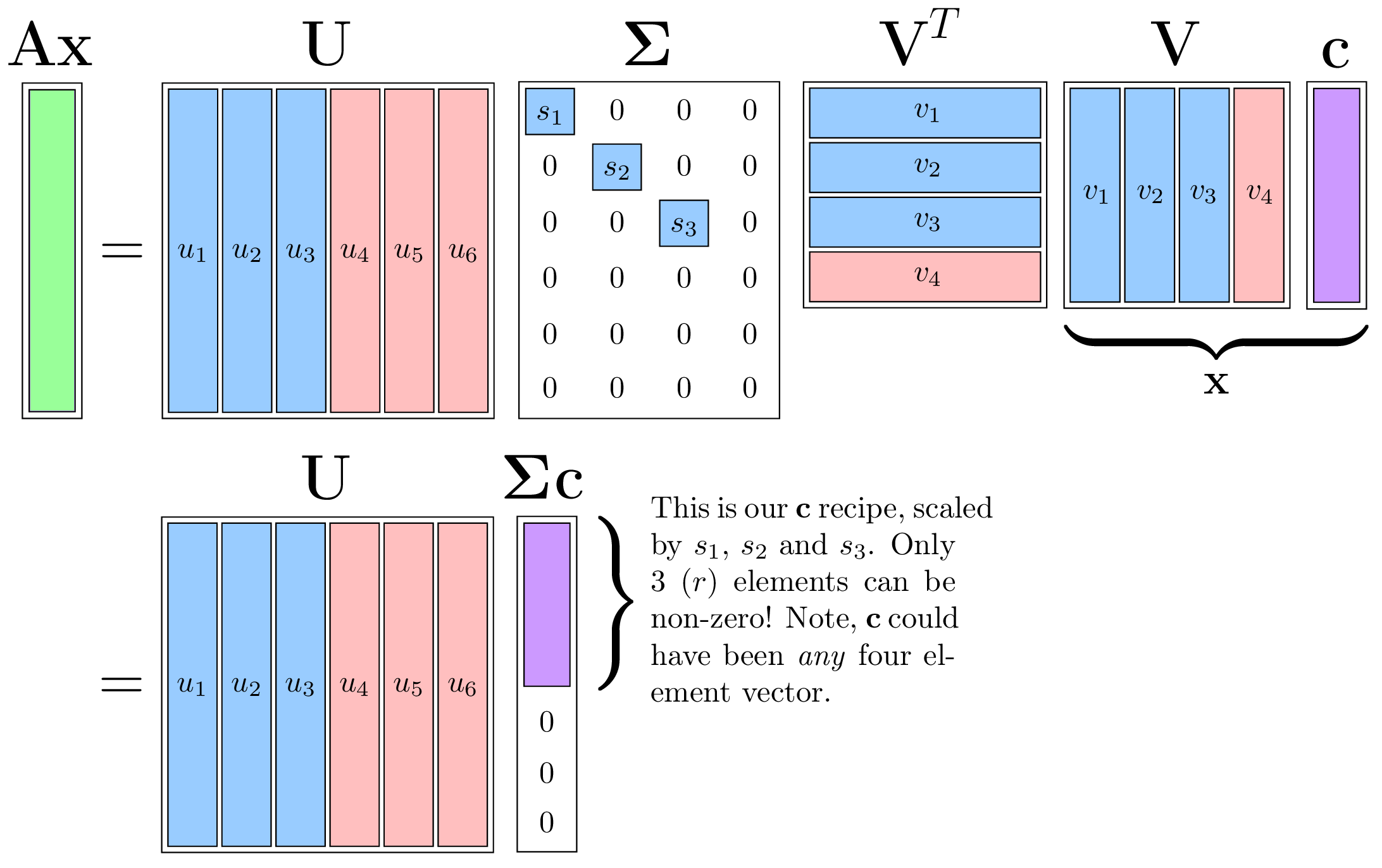
We see \(\boldsymbol{\Sigma}\mathbf{c}\) is just the \(\mathbf{x}\) recipe scaled element-wise by the singular values, leaving only three (\(r\)) non-zero values. With this readjusted recipe, the output \(\mathbf{U}\boldsymbol{\Sigma}\mathbf{c}\) is just the recipe applied, but with the ingredients as \(\mathbf{U}\)’s columns.
I’ll say that differently. \(\mathbf{Ax}\) is a linear combination of the left singular vectors where that combination is determined by:
- The recipe for making \(\mathbf{x}\) out of the right singular vectors. So if \(\mathbf{x}\) is made up a lot of \(\mathbf{v}_2\), then the output will have a lot of \(\mathbf{u}_2\).
- The singular values, which scale or eliminate elements of \(\mathbf{c}\).
That’s the main idea, but it’s part of a bigger picture.
The Fundamental Theorem of Linear Algebra
Baked into this is an important connection.
SVD tells us how the row space (all vectors constructable with the rows of \(\mathbf{A}\)) relates to the column space (all vectors constructable with the columns).
Ultimately, it comes down to the rank \(r\). It reflects the dimension of both the column space and the row space. Using the example above, there are only three (\(r\)) dimensions (those of the row space) within the four dimensions that \(\mathbf{x}\) lives, whereby movements will result in movements in the output \(\mathbf{Ax}\), which consequently can only move in three dimensions (those of the column space). Consider two vectors \(\mathbf{x}_1\) and \(\mathbf{x}_2\), which have recipes \(\mathbf{c}_1\) and \(\mathbf{c}_2\) that differ only on their loading for \(\mathbf{v}_4\). Their outputs \(\mathbf{Ax}_1\) and \(\mathbf{Ax}_2\) would be the same because that loading is multiplied by zero. That dimension does not matter. In fact, that space, the one dimensional line along \(\mathbf{v}_4\), has a name: the null space of \(\mathbf{A}\).
We’ve now accounted for all four dimensions where \(\mathbf{x}\) lives. We should do the same for all dimension of \(\mathcal{R}^6\). We know the output \(\mathbf{Ax}\) must be a linear combination of the first three (blue) columns of \(\mathbf{U}\) and therefore, can only move in three dimensions. The remaining three dimensions can be thought of as the ‘unreachable’ subspace of \(\mathcal{R}^6\); we can’t choose any \(\mathbf{x}\) such that the output will land in this space. We call this the null space of \(\mathbf{A}^{\top}\).
By categorizing the dimensions of \(\mathcal{R}^4\) and \(\mathcal{R}^6\) as named subspaced, we’ve accounted for all dimensions. More formally:
- null space of \(\mathbf{A}\), labeled \(\textrm{Null}(\mathbf{A})\): subspace of \(\mathcal{R}^4\) where movements make no difference in the output \(\mathbf{Ax}\). Think of it as the ‘Doesn’t Matter’ space.
- column space of \(\mathbf{A}\), labeled \(\textrm{Col}(\mathbf{A})\): subspace of \(\mathcal{R}^6\) where \(\mathbf{Ax}\) could land with a properly chosen \(\mathbf{x}\). Think of it as the ‘Reachable’ space.
- null space of \(\mathbf{A}^{\top}\), labeled \(\textrm{Null}(\mathbf{A}^{\top})\): subspace of \(\mathcal{R}^6\) where \(\mathbf{Ax}\) could never land. Think of it as the ‘Unreachable’ space.
- row space of \(\mathbf{A}\), which is also the column space of \(\mathbf{A}^{\top}\), so its labeled \(\textrm{Col}(\mathbf{A}^{\top})\): subspace of \(\mathcal{R}^4\) which drives the difference in \(\mathbf{Ax}\). Think of it as the ‘Matters’ space.
For intuition, we may think of this relation graphically. It’ll help to consider \(\mathbf{x}\) as made up of two parts, that which exists in \(\textrm{Col}(\mathbf{A}^{\top}\)), labeled \(\mathbf{x}_r\), and that which exists in \(\textrm{Null}(\mathbf{A}\)), labeled \(\mathbf{x}_n\). Therefore \(\mathbf{x}=\mathbf{x}_n+\mathbf{x}_r\). This separation is well defined due to the orthogonality of the subspaces’ basis vectors, and that orthogonality is emphasized with the right-angle touch of red and blue seen below.
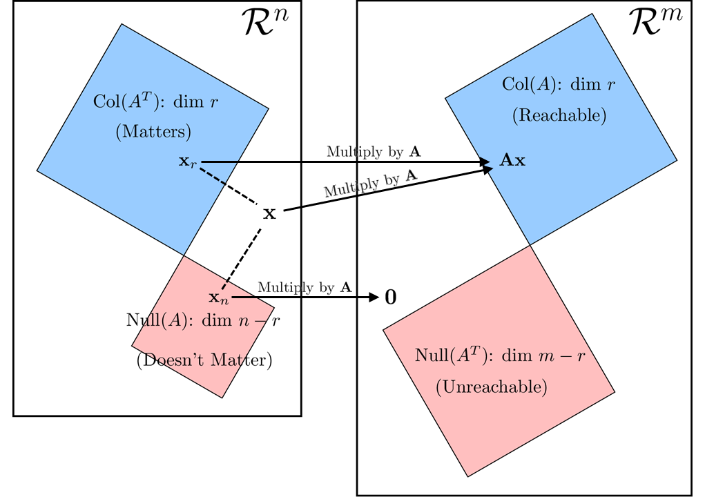
The relationship of subspaces when considering \(\mathbf{Ax}\) \(\\\)This is a close imitation of figure 1 from Strang (1993).
We see that \(\mathbf{Ax}\) and \(\mathbf{Ax}_r\) map to the same point. Only the piece of \(\mathbf{x}\) that resides in the column space of \(\mathbf{A}^{\top}\) matters for determining its output, as described earlier.
Next, what if we consider a point \(\mathbf{y}\) in \(\mathcal{R}^6\) and apply \(\mathbf{A}^{\top}\) to get \(\mathbf{A}^{\top}\mathbf{y}\)? In that case, all these subspaces remain and we have a familiar, reversed relation:
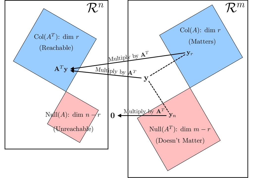
The relationship of subspaces when considering \(\mathbf{A}^{\top}\mathbf{y}\) \(\\\)This is a close imitation of figure 1 from Strang (1993).
Comparing these two graphics, we see the equivalence:
- The ‘Unreachable’ space with multiplication by \(\mathbf{A}\) is the ‘Doesn’t matter’ space for multiplication by \(\mathbf{A}^{\top}\) and visa versa.
- The ‘Matters’ space for multiplication by \(\mathbf{A}\) is the ‘Reachable’ space for multiplication by \(\mathbf{A}^{\top}\) and visa versa.
And it is this symmetry that explains the subspace labeling. Upon considering only multiplication by \(\mathbf{A}\), the labels \(\textrm{Null}(\mathbf{A})\), \(\textrm{Col}(\mathbf{A})\), \(\textrm{Null}(\mathbf{A}^{\top})\) and \(\textrm{Col}(\mathbf{A}^{\top}\)) appear surprisingly reductive. They reflect only two types of spaces, \(\textrm{Null}(\cdot)\) and \(\textrm{Col}(\cdot)\), when four types have been described: ‘Matters’, ‘Doesn’t Matter’, ‘Reachable’ and ‘Unreachable’. Ultimately, however, we realize these four are produced by considering \(\textrm{Null}(\cdot)\) and \(\textrm{Col}(\cdot)\) of both transformations \(\mathbf{Ax}\) and \(\mathbf{A}^{\top}\mathbf{y}\).
In Summary
SVD tells us how to decompose a matrix into sets of orthonormal vectors which span \(\mathcal{R}^n\) and \(\mathcal{R}^m\). Depending on the singular values these are paired with, we know what subspace of \(\mathcal{R}^n\) matters for driving \(\mathbf{Ax}\) within the reachable space of \(\mathcal{R}^m\). Specifically, \(\mathbf{Ax}\) will be a linear combination of the spanning vectors of the ‘Reachable’ space where that combination depends on the singular values and the recipe for making \(\mathbf{x}\) out of the spanning vectors of the ‘Matters’ space. That connection forces the dimensionality of these spaces to be the same. A consideration of multiplication by \(\mathbf{A}^{\top}\) reveals that we may think of ‘Reachable’ spaces as ‘Matters’ spaces and ‘Unreachable’ as ‘Doesn’t Matter’ if we view it in the opposite direction.
References
-
G. Strang. The Fundamental Theorem of Linear Algebra. The American Mathematical Monthly Vol. 100 No. 9. Nov 1993.
-
K. Murphy. Machine Learning: A Probabilistic Perspective. MIT Press. 2012.
Something to Add?
If you see an error, egregious omission, something confusing or something worth adding, please email dj@truetheta.io with your suggestion. If it’s substantive, you’ll be credited. Thank you in advance!
Footnotes
-
See section 12.2 of Murphy (2012) for more information on this statement of SVD. ↩