The Trace as a Measure of Complexity

By: DJ Rich

Posted: February 22, 2018 Updated: September 19, 2023

The trace of a square matrix, the sum of the diagonal entries, turns out to be useful for model selection:

The trace quantifies complexity for a certain class of model.

If two models explain the data equally well, then the conventional wisdom is to pick the simpler one. But what if one is much simpler but explains the data only slightly less well?

This raises the question of how to weigh model complexity against its ability to fit the data. And to weight is to quantify. As we’ll see, the trace provides an especially simple and intuitive quantification.

The Class of Models

The class of models referred to is any in which the fitted values can be produced as:

\[\hat{\mathbf{y}} = \mathbf{S}\mathbf{y}\]

Some familiar models take this form:

OLS Regression with a design matrix $\mathbf{X}$: $~$\begin{align}\mathbf{S} = \mathbf{X}\big(\mathbf{X}^T\mathbf{X}\big)^{-1}\mathbf{X}^T\end{align}$~$
Ridge Regression: $~$\begin{align}\mathbf{S} = \mathbf{X}\big(\mathbf{X}^T\mathbf{X}+\lambda\mathbf{I}\big)^{-1}\mathbf{X}^T\end{align}$~$ where $\lambda$ is a hyperparameter to be selected by the modeler.
Applying a natural cubic spline: $~$\begin{align}\mathbf{\hat{y}} = \mathbf{S}_\lambda\mathbf{y}\end{align}$~$ where $\mathbf{S}_\lambda$ is the natural cubic spline’s smoothing matrix.

Essentially, models of this form are linear, in that predictions are linear combinations of observed $y$’s.

An Experiment for Measuring Complexity

How can we quantify complexity in the general “$\mathbf{\hat{y}} = \mathbf{S}\mathbf{y}$” case? If we were given two models represented as $\mathbf{S}^{(A)}$ and $\mathbf{S}^{(B)}$, what experiment could we run to determine which is more complex?

In essence, a complex model can fit a larger range of patterns than a simple one can. If a complex model is given some $\mathbf{y}$, it’ll better reproduce it than a simple one will.

This motivates the following experiment. It begins with an assumption of how $\mathbf{y}$ is generated:

$~$\begin{align} y_i = g(\mathbf{x}_i) + \epsilon_i \end{align}$~$

where $g(\cdot)$ is a true-and-unknown function, $\mathbf{x}_i$ is a feature vector¹ and $\epsilon_i$ is some mean-zero noise with variance $\sigma^2_\epsilon$. We’ll generate many $\mathbf{y}$’s from this, deliver them to the two models and observe the outgoing streams of fitted values. As per our intuition on complexity, we should inspect how well each model recreates its given $\mathbf{y}$.

To do that, we look at one element of $\mathbf{y}$; we’ll view the scatter plot of the model’s inputs-outputs² for that element. We can do this for a few randomly selected elements:

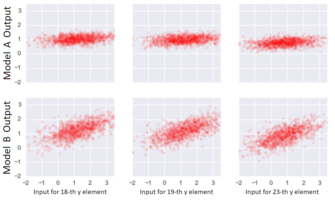Alt Scatter plots between $y_i$ and $\hat{y}_i$ for three $i$’s and two models. Each point corresponds to one sampling from the true data generating mechanism and the associated fitted value.

We see that model $B$ is more sensitive to inputs. This sensitivity is exactly what we mean by complexity.

A complex model is one where $\hat{y}_i$ is very sensitive to $y_i$, since this sensitivity is required for close reproduction of $y_i$.

To quantify, we measure sensitivity with the slope of the best fit line³. We label it $\beta_i$ and it can be viewed as:

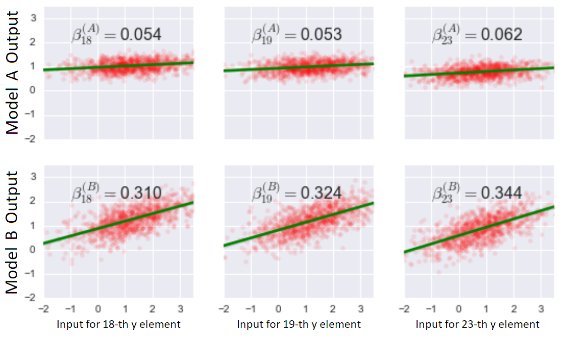Alt We see that the more complex model has a larger correlation between observed $y_i$’s and fitted $\hat{y}_i$’s.

On a per-element basis, we now have a measure of complexity. How should we combine these into a measure for the full model? Suppose both models yield the same input-output $\beta_i$’s, but the first model only applies to a $\mathbf{y}$ vector of length 10, whereas the second works for a vector of length 1,000. Insofar as the latter is 100 $\times$ more of a pattern to match than the former, so should the model complexity scale. This suggests:

The model’s complexity is the sum of $\beta_i$’s:
\[\begin{align} \textrm{Complexity}(\mathbf{S}) = \sum_i \beta_i \end{align}\]

Measuring Complexity in Practice

As presented, this measure comes from the inaccessible world where $\mathbf{y}$’s can be repeatedly sampled. How do we actually measure complexity without experimenting with the true-and-unknown data generating process?

Since complexity is a function of the model alone, we should be able to measure it using only $\mathbf{S}$. To do so, we note the following:

\[\begin{align} \beta_i = \frac{\textrm{cov}(\hat{y}_i,y_i)}{\textrm{var}(y_i)} = \frac{\textrm{cov}(\hat{y}_i,y_i)}{\sigma^2_\epsilon} \end{align}\]

Since $\hat{y}_i$ is a linear combination of $\mathbf{y}$, we may write:

\[\begin{align} \frac{\textrm{cov}(\hat{y}_i,y_i)}{\sigma^2_\epsilon} & = \frac{\textrm{cov}(s_{i1}y_1+s_{i2}y_2+\cdots+s_{iN}y_N,y_i)}{\sigma^2_\epsilon} \\ & = \frac{s_{ii}\textrm{var}(y_i)}{\sigma^2_\epsilon} \\ & = s_{ii} \end{align}\]

where $s_{ij}$ is the element of $\mathbf{S}$ at the $i$-th row and $j$-th column. For the full model, this means:

$~$\begin{align} \textrm{Complexity}(\mathbf{S}) = \sum_i s_{ii} = \textrm{Trace}(\mathbf{S}) \end{align}$~$

And there we have it; the trace of a linear model is a measure of complexity. It is often called the effective degrees of freedom. Intuitively, it measures how much a model uses $y_i$ in its recreation of $\hat{y}_i$.

In the case of the two example models, their complexities were:

\[\begin{align} \textrm{Trace}(\mathbf{S}^{(A)}) &= 5 \\ \textrm{Trace}(\mathbf{S}^{(B)}) &= 23 \end{align}\]

We can observe this by inspecting fits for a randomly selected $\mathbf{y}$:

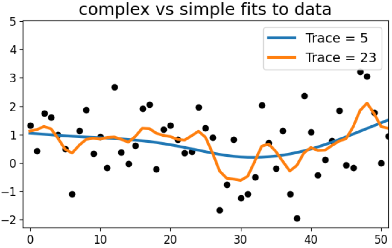Alt The more complex model is better at matching the fluctuations of a given $\mathbf{y}$. The simpler model can’t follow as closely and performs more aggressive smoothing, which may be better for out of sample predictions.

Place it on the scale

With this complexity quantifier, we can form a fitness-vs-complexity objective, used to determine $\mathbf{S}$. It can be expressed generally as:

$~$\begin{align}\textrm{(fit to the data)} + \lambda\textrm{(model complexity)}\end{align}$~$

where $\lambda$ is some fitness-vs-complexity hyperparameter, to be determined by the modeler⁴. More specifically, we might determine the $\mathbf{S}$ that minimizes:

$~$\begin{align}(\mathbf{y} - \mathbf{S}\mathbf{y})^T(\mathbf{y} - \mathbf{S}\mathbf{y}) + \lambda\textrm{Trace}(\mathbf{S})\end{align}$~$

This isn’t typically how such objectives are written, because we often know more about $\mathbf{S}$ which simplifies the trace expression⁵. Still, this is equivalent and captures the general case.

‘Free’ Complexity

It’s worth noting that Trace$(\mathbf{S})$ ignores everything off the diagonal of $\mathbf{S}$. Such values can be anything and it’ll make no difference to the complexity measure. That is, there is no complexity cost for large magnitude coefficients if they are used to construct $\hat{y}_i$ from $\{y_j : j \neq i\}$. This is reminiscent of leave-one-out cross validation, where the recommendation is: ‘pick any model, regardless of its complexity, that best predicts $y_i$ when given a training set that excludes $y_i$.’

References

T. Hastie, R. Tibshirani and J. H. Friedman. The Elements of Statistical Learning: Data Mining, Inference, and Prediction 2nd ed. New York: Springer. 2009.

Something to Add?

If you see an error, egregious omission, something confusing or something worth adding, please email dj@truetheta.io with your suggestion. If it’s substantive, you’ll be credited. Thank you in advance!

Footnotes

The features will not appear explicitly in the model. Rather, they are implicitly included in $\mathbf{S}$. ↩
In this case, the inputs refer to $\mathbf{y}$ and the outputs refer to $\hat{\mathbf{y}}$. This is not to be confused with common case where $\mathbf{x}_i$ are refered to as inputs. ↩
One could technically have a model that has a sensitivity greater than 1, but that would certainly hurt the fit. ↩
To optimize a choice of $\lambda$ is to search along the bias-variance trade-off, where a model is found that balances capturing patterns against ignoring noise. Such balance is essential for predicting well out of sample. ↩
To see for yourself, try the case for linear regression and use SVD on $\mathbf{X}$. ↩

Share on

Twitter Facebook LinkedIn

Writing