Information Theory and Entropy
Posted: Updated:
As defined within information theory, entropy is an elegant answer to a baffling question:
How is information measured?
To approach this, we’ll begin with the definition and display of entropy. This will reveal its mechanics and that it’s merely a short computation on a distribution.
We’ll come to appreciate it when we extend it to two variables. We’ll motivate by reasoning from extremes and find a remarkable structure emerge, a structure which can be manipulated by analogy to something simpler. In the end, we’ll have multiple quantifications of information and a means to reason about them that involves no algebraic overhead.
What is Entropy?
We consider entropy for a discrete1 random variable \(X\). Precisely, a sample of \(X\) can be any value \(x\) from the set \(\mathcal{X}\) with probability \(p(x)\). If there are \(N\) values in the set \(\mathcal{X}\), this may represented as:
 a generic representation of a discrete random variable distribution \(\\\) The second column represents discrete values the variable may take and the third column represents their probabilities.
Entropy measures a distribution’s uncertainty. If \(X\) has high entropy, it is highly uncertain. It is defined as:
\[\mathbb{H}(X) = \sum_{i=1}^{N} p(x_i) \log_2 \frac{1}{p(x_i)}\]
Interestingly, uncertainty and information are two sides of the same coin; if we are highly uncertain of an event before it happens, then observing it is highly informative.
This can be understood (merely descriptively) by reasoning from extremes. By intuition, consider what constitutes an uninformation event; that is one which is likely, an event expected to happen. To discover an event likely to happen in fact happened is to discover very little. By the same logic, an informative event is a rare, unexpected event. Observing something rare and unexpected has potential to strongly update beliefs, which is akin to acquiring information2. In total, a random variable is informative if its average outcome is rare, and therefore, hard to predict and highly uncertain. Stated differently:
Observing an uncertain, hard-to-predict event provides more information than observing a certain, easy-to-predict one.
As an aside, this suggests a useful heuristic: If we are to design an experiment to learn something, it should be designed such that aprior, we are most uncertain about its outcome. If so, observing it will be the most informative. This makes claim to a huge decision space, and so isn’t a perfect rule. But it can be a surprising shortcut to otherwise difficult problems; see pages 68-70 of MacKay (2003) for such a case.
We must also mention entropy’s original context, communication across a noisy channel. Such communication involves streaming 0’s and 1’s from one end to the other, where bits may be randomly flipped with some fixed probability. To avoid the topic’s depth, we consider a noiseless channel and ask about encoding observations of \(X\) across the channel. For instance, if \(X\) is a uniform distribution over the alphabet \(\{\textrm{a}, \textrm{b}, \cdots, \textrm{z}\}\), one might encode each letter as a string of five bits. For example, if ‘\(\,\textrm{c}\,\)’ and ‘\(\,\textrm{f}\,\)’ are encoded as \(00101\) and \(10100\) respectively, then passing \(0010110100\) communicates ‘\(\,\textrm{cf}\,\)’. From here, we can alternatively describe entropy:
\(\mathbb{H}[X]\) is the smallest average bit-length per \(x_i\) achievable with a noiseless channel and knowledge of \(p(x)\).
Understandably, describing entropy this way seldom evokes a comfortable response. It’s hard to operationalize. What are typical values of \(\mathbb{H}[X]\)? How does \(\mathbb{H}[X]\) change as \(p(x)\) changes? Fortunately, there are simpler perspectives, like inspecting its mechanical behavior.
The Mechanics of Entropy
Notice entropy doesn’t care about the \(x_i\) values. It only considers their probabilities \(p(x_i)\)3. Among other benefits, this lets us fully represent the distribution with a sorted bar graph where the horizontal axis is the index \(i\), the height of each bar is \(p(x_i)\) and bars are sorted in increasing order. The bar graph represents a distribution in precisely the way entropy cares; if two distributions produce the same sorted bar graph, they’ll have equal entropy.
To feel the mechanics, we vary bar graphs in two ways:
- Increase N. How does entropy respond as we increase the number of values \(X\) may take?
- Decrease the concentration of probability. In one extreme, all \(p(x_i)\)’s are equal and in the other, a few \(x_i\)’s contain the majority of the probability mass.
Exploring these gives the following:
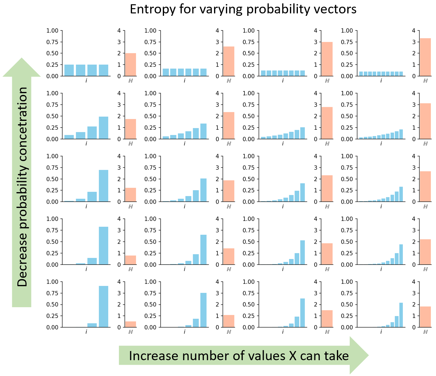
So we see:
Entropy increases as the count of possible values increases and as the probability mass spreads out.
But at this level, its properties can’t be appreciated. To change that, we consider the following.
Entropy of a Bivariate Joint Distribution
Consider two random variables \(X\) and \(Y\) along with their joint distribution. We again may imagine them as grids:
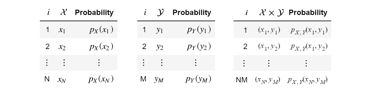 Generic marginal and joint distributions of \(X\) and \(Y\) may be thought of as grids.
Before we define the entropy of both \(X\) and \(Y\), denoted \(\mathbb{H}[X,Y]\), we ask: How should it relate to \(\mathbb{H}[X]\) and \(\mathbb{H}[Y]\)? If we keep in mind that entropy seeks to measure information as uncertainty, we can intuit:
- If \(X\) and \(Y\) are related by a known invertible function, then knowing one is as good as knowing the other. That is, after observing one, no information is gained with observing the other. This suggests the information of both is the information of either of them, which is the same:
- Conversely, if \(X\) and \(Y\) are independent, observing one provides no information regarding the other. In this sense, they represent distinct sources of information. Therefore, information of both must be the sum of their individual information4:
We see that at opposite extremes, perfect dependence and perfect independence, claims can be made about a natural quantification of information. When inspecting these claims, it seems we’re dealing with volumes. The following visual comes to mind:
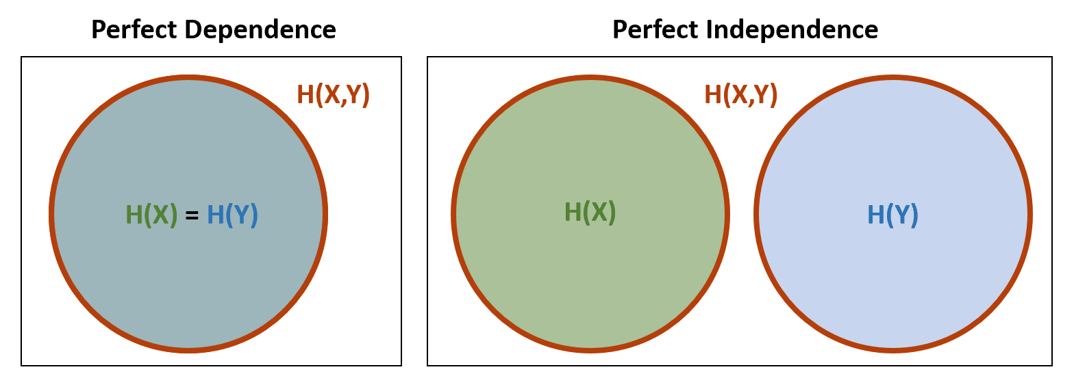 Entropy of \(X\) and \(Y\) are depicted at two extremes, perfect dependence and perfect independence.
From here, a natural and fruitful idea is to imagine the middle ground:
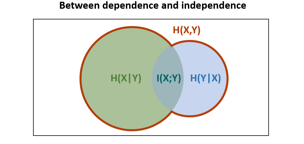 the relationship of \(\mathbb{H}[X]\), \(\mathbb{H}[Y]\) and \(\mathbb{H}[X,Y]\) where \(X\) and \(Y\) share a source of information \(\\\) Depiction originated in Yeung (1991)
This creates three new quantities to ponder, labeled in anticipation as \(\mathbb{H}[X \vert Y]\), \(\mathbb{H}[Y \vert X]\) and \(\mathbb{I}[X;Y]\). It turns out, remarkably, these quanties correspond to independently legitimate measures of information, and by this visual aid, we may conceptualize their relation merely as overlapping areas. It’s not a perfect analogy (see pages 143-144 of MacKay (2003) for more), but it has its merits, as we’ll see. For a complete discussion and the generalization to three variables, see Yeung (1991).
For now, we define the quantities from the graphic.
Conditional Entropy
The leftmost region, labeled \(\mathbb{H}[X \vert Y]\), is the conditional entropy of \(X\) given \(Y\). It’s defined as:
\[\mathbb{H}[X \vert Y] = \sum_{j=1}^{M} \mathbb{H}(X \vert Y=y_j)p_Y(y_j)\]It quantifies the uncertainty of \(X\) remaining after observations of \(Y\). If \(X\) and \(Y\) share information, then an observation of \(y\) allows one to create a distribution over \(X\) with reduced uncertainty. If the reduced entropies, labeled \(\mathbb{H}(X \vert Y=y_j)\), are averaged and weighed by their probabilities \(p_Y(y_j)\), we obtain \(\mathbb{H}[X \vert Y]\). This is symmetrically true for \(\mathbb{H}[Y \vert X]\).
Intuitively, as a minimum average bit length captures uncertainty, it measures the remaining bit length if the sender and receiver are simulatenously aided with an observation of a related variable \(y_j\).
Mutual Information
The overlapping region, labeled \(\mathbb{I}[X;Y]\), is the mutual information of \(X\) and \(Y\). It is defined as:
\[\mathbb{I}[X;Y] = \sum_i^N \sum_j^M p_{X,Y}(x_i,y_j) \log\big(\frac{p_{X,Y}(x_i,y_j)}{p_X(x_i)p_Y(y_j)}\big)\]We can avoid a direct interpretation of this expression. It is easier to think in terms of KL divergence, a distance-like measure between probability distributions. All that is necessary to know is that identical distributions have a KL divergence of 0 and very dissimilar ones yield a large positive value.
Mutual information is the KL divergence between the joint distribution \(p_{X,Y}(x_i,y_j)\) and an approximation of the joint made by a product of the marginal distributions, \(p_X(x_i)p_Y(y_j)\). Such an approximation is, by an information theoretic perspective, the best approximation one can make when \(X\) and \(Y\) are forced to be independent.
From this, we may reason:
- If \(\mathbb{I}[X;Y] = 0\), the product is a perfect approximation, and so \(p_{X,Y}(x_i,y_j) = p_X(x_i)p_Y(y_j)\). We see this implies their independence.
- If \(\mathbb{I}[X;Y]\) is high, on average \(p_{X,Y}(x_i,y_j)\) looks very different from \(p_X(x_i)p_Y(y_j)\), so it’s very not-independent; they are very dependent.
This matches the reasoning by extremes we did earlier. If the \(\mathbb{I}[X;Y]\) region is large, that is the high dependency case. If it’s zero, that is the independent case.
No Algebraic Overhead
At this point, we know \(\mathbb{H}[X,Y]\), \(\mathbb{H}[X]\), \(\mathbb{H}[Y]\), \(\mathbb{H}[Y \vert X]\), \(\mathbb{H}[X \vert Y]\) and \(\mathbb{I}[X;Y]\) are independently useful quantifications of information under different circumstances. If one were interested in these measures but knew only their formula, reasoning about their relationships would be difficult.
But if we understand their analogy to overlapping areas, manipulations become easy. From the visual, we can deduce:
\[\begin{align*} \mathbb{H}[X,Y] & = \mathbb{H}[X] + \mathbb{H}[Y] - \mathbb{I}[X;Y] \\ \mathbb{H}[X,Y] & = \mathbb{H}[X] + \mathbb{H}[Y \vert X] \\ \mathbb{H}[X,Y] & = \mathbb{H}[X \vert Y] + \mathbb{H}[Y \vert X] + \mathbb{I}[X;Y] \\ \mathbb{I}[X;Y] & = \mathbb{H}[Y] - \mathbb{H}[Y \vert X] \\ \mathbb{H}[X] & \geq \mathbb{H}[X \vert Y] \\ \end{align*}\]And if one were to do the laborious calculations, all of these are true!
Further, the above analogizes operations. To know a random variable is to subtract its information from the uncertainty of another.
This perspective makes the topic far easier to internalize. On a subjective note, I find the analogy to be a stunning example of mathematical elegance, where something abstract and removed reduced cleanly to something simple and familiar.
References
Chapter 2 from Cover et al. (2006) and chapter 8 from MacKay (2003) were primary sources.
-
T. M. Cover and J. A. Thomas. The Elements of Information Theory, 2nd Edition. Wiley-Interscience. 2006.
-
D. MacKay. Information Theory, Inference and Learning Algorithms. Cambridge University Press. 2003.
-
Wikipedia contributors. Mutual Information. Wikipedia, The Free Encyclopedia.
-
R. W. Yeung. A New Outlook on Shannon-Information Measures. IEEE Trans. Info. Theory 37. 1991.
Something to Add?
If you see an error, egregious omission, something confusing or something worth adding, please email dj@truetheta.io with your suggestion. If it’s substantive, you’ll be credited. Thank you in advance!
Footnotes
-
Entropy can be extended to continuous variable as differential entropy, but some of its properties are lost. ↩
-
Per information theory, we quantifiably gain \(\log_2 \frac{1}{p(x_i)}\) bits of information when observing the event \(x_i\). For example, if observing an event gives 3 bits of information, this suggest it provides the same information content of answering a question where all answers are equally likely and can be coded by 3 bit strings, of which there are 8. In comparison, answering a question with 4 equally likely answers is less informative (by 1 bit). ↩
-
Contrast this with another measure of uncertainty variance, which does care about the \(x_i\)-values. ↩
-
In fact, the connection between independence and summation establishes the use of the logarithmic function \(\log_2(\cdot)\), since independence definitionally exists when joint probabilities equal the product of marginal probabilities and \(\log_2(\cdot)\) turns products into sums. ↩