Part 1: An Introduction to Probabilistic Graphical Models
Posted: Updated:
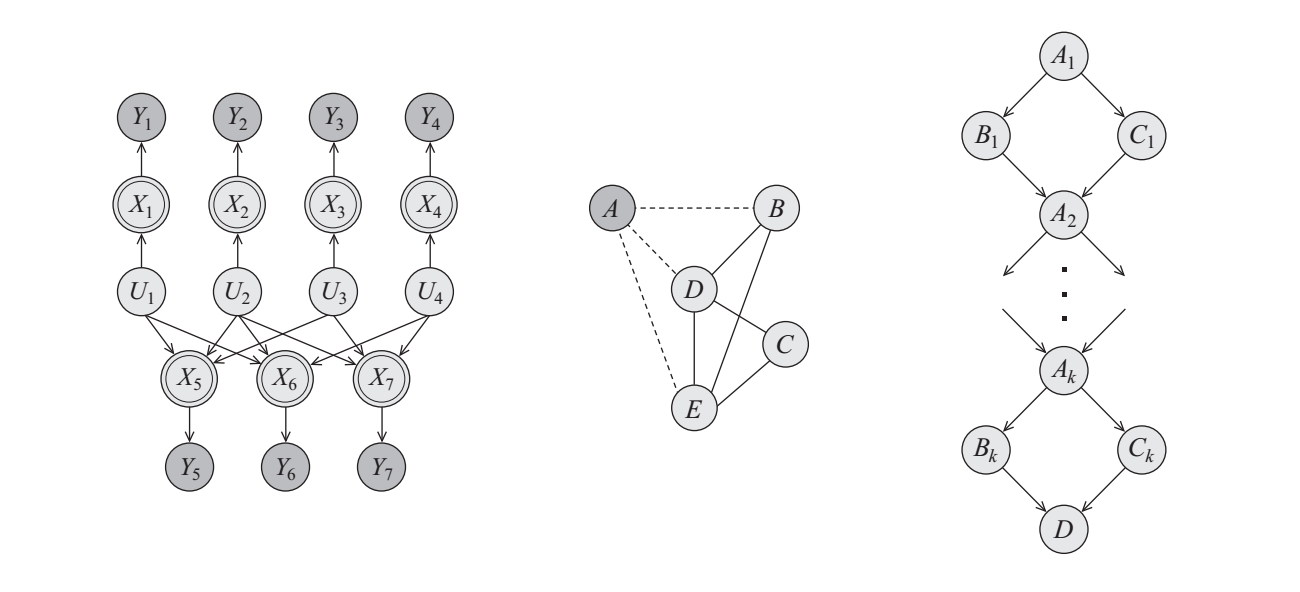 Probabilistic Graphical Models. These images are from Probabilistic Graphical Models by Koller and Friedman and used with permission.
These are Probabilistic Graphical Models (‘PGMs’). Among the diversity of computational models, PGMs are exceptional for their synthesis of probability theory and graph theory. They have proven valuable tools for managing the otherwise baffling mixture of uncertainty and complexity nature so often presents. Whether it’s deciphering the tangled web of genes in bioinformatics or inferring human behavior in social networks, PGMs have contributed in both scientific research and real-world applications1.
This post is to introduce a seven part series covering the basics:
- Part 1: An Introduction to Probabilistic Graphical Models
- Part 2: Exact Inference
- Part 3: Variational Inference
- Part 4: Monte Carlo Methods
- Part 5: Learning Parameters of a Bayesian Network
- Part 6: Learning Parameters of a Markov Network
- Part 7: Structure Learning
To ease digestion, the dependencies can be understood with a map:
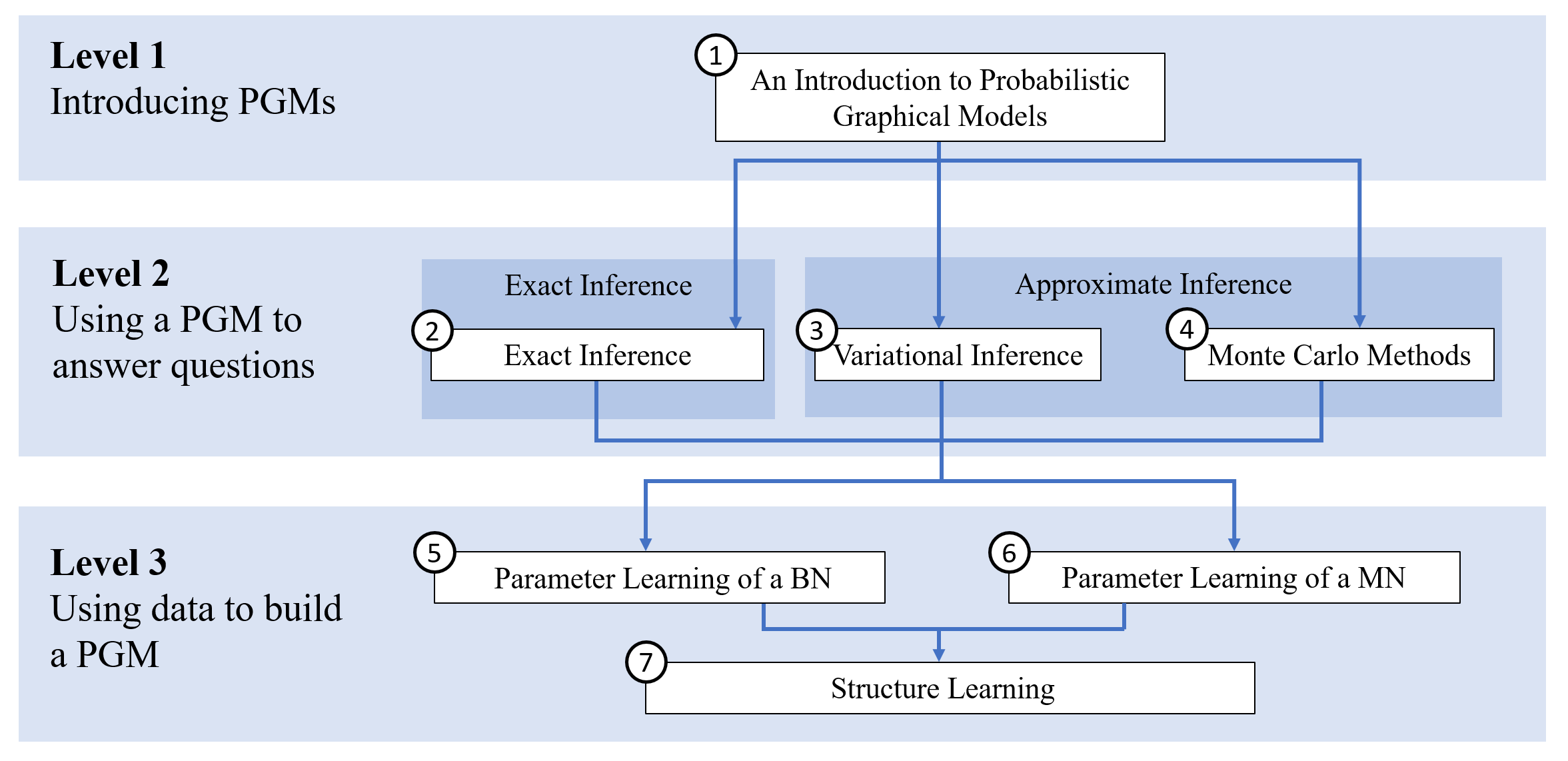 Dependencies among topics
Parts within the same level do not depend on each other. One could read the path \(1 \rightarrow 2 \rightarrow 6 \rightarrow 7\) and would never be without the proper context. To refresh concepts, each post points to summaries of prerequisites posts.
I first wrote this series in 2018, following my study of Probabilistic Graphical Models by Daphne Koller and Nir Friedman. I’ve updated it in 2023, following four years of applying causal graphical models at Lyft to help manage their driver and rider market2. My intent is to briefly tour the subject, emphasize its principles and potentially assist an application by the reader.
To caveat, this is by no standard comprehensive. Anyone seeking a deep and wide understanding should refer to Koller and Friedman’s text, this series’ primary source. What they have collected, discovered and expressed as a consistent set of principles is a remarkable feat. Further, Kevin Murphy’s Machine Learning: A Probabilistic Perspective was frequently relevant as well and is, for topics outside PGMs, worthy of similar praise.
Before we begin, it’ll help to review the Notation Guide. Then we ask:
What Problem does a PGM Address?
Our goal is to understand a complex system. We assume the system manifests as \(n\) random variables3, denoted as \(\mathcal{X} = \{X_1,X_2,\cdots,X_n\}\)4, and is governed by a joint distribution \(P\). Here, to ‘understand’ means we can answer two categories of questions accurately and efficiently. If \(\mathbf{Y}\) and \(\mathbf{E}\) are subsets of \(\mathcal{X}\), the categories are:
- Probability Queries: Compute the probabilities \(P(\mathbf{Y} \vert \mathbf{E}=\mathbf{e})\). That is, what is the distribution of \(\mathbf{Y}\) given some observation of the random variables of \(\mathbf{E}\)?
- MAP Queries: Determine \(\textrm{argmax}_\mathbf{Y}P(\mathbf{Y} \vert \mathbf{E}=\mathbf{e})\). That is, determine the most likely joint assignment of one set of random variables given a joint assignment of another.
It’s worth noting:
- Since \(\mathbf{Y}\) and \(\mathbf{E}\) are any two subsets of \(\mathcal{X}\), there is potentially a remaining set: \(\mathbf{Z} = \mathcal{X} - \{\mathbf{Y},\mathbf{E}\}\). This set is omitted in the notation but strongly at play. We must sum them out, which can considerably increase compute. For example, \(P(\mathbf{y} \vert \mathbf{e})\) is in fact \(\sum_\mathbf{Z}P(\mathbf{y},\mathbf{Z} \vert \mathbf{e})\).
- There is no reference to a model; we are only asking for probabilities and values that accurately track the system of \(\mathcal{X}\).
Further, we are assisted with some, at least partial, observations of \(\mathcal{X}\).
The Problem with Large Joint Distributions
The starting point, perhaps surprisingly, is to assume \(P\) is known. This is not the case in practice but reveals essential facts.
We may think of \(P\) as a table that lists all joint assignments of \(\mathcal{X}\) and their probabilities. If \(\mathcal{X}\) is made up of 10 random variables, each of which can take 1 of 100 values, the table has \(100^{10}\) rows, each indicating an assignment of \(\mathcal{X}\) and its probability.
The problem is, for a complex system, this table is exponentially large. Even if we knew \(P\), we could not run computations on it. To overcome this, we need the following concept, fundamental to PGMs.
The Conditional Independence Statement
We need a compact representation of \(P\), something that provides access to its contents but doesn’t requiring writing its table down. To this end, we have the Conditional Independence (CI) statement:
Given subsets of random variables \(\mathbf{X}\), \(\mathbf{Y}\) and \(\mathbf{Z}\) from \(\mathcal{X}\), we say \(\mathbf{X}\) is conditionally independent of \(\mathbf{Y}\) given \(\mathbf{Z}\) if
\[P(\mathbf{x},\mathbf{y} \vert \mathbf{z})=P(\mathbf{x} \vert \mathbf{z})P(\mathbf{y} \vert \mathbf{z})\]for all \(\mathbf{x}\in \textrm{Val}(\mathbf{X})\), \(\mathbf{y}\in \textrm{Val}(\mathbf{Y})\) and \(\mathbf{z}\in \textrm{Val}(\mathbf{Z})\).
This is stated as ‘\(P\) satisfies \((\mathbf{X}\perp \mathbf{Y} \vert \mathbf{Z})\).’
If we had sufficient compute, we could calculate the left and right side for a distribution \(P\). If the equation holds for all values, the CI statement holds by definition.
Intuitively, though not obviously, a CI statement implies the following. If we are given the assignment of \(\mathbf{Z}\), then knowing the assignment of \(\mathbf{X}\) will never help us guess \(\mathbf{Y}\) (and vice versa). In other words, \(\mathbf{X}\) provides no information for predicting \(\mathbf{Y}\) beyond what is within \(\mathbf{Z}\). Equivalently, we can’t predict \(\mathbf{X}\) from \(\mathbf{Y}\) given \(\mathbf{Z}\).
Crucially, CI statements enable a compact representation of \(P\). To see this, suppose \((X_i \perp X_j)\) for all \(i \in \{1,\cdots,10\}\) and \(j \in \{1,\cdots,10\}\) where \(i\neq j\). This is to say, all random variables are independent of all other random variables. With this, we only need to know the marginal probabilities for each random variable (using the previous example, this involves a total of \(10\cdot 100=1000\) numbers) to reproduce all probabilities of \(P\). For instance, if we are considering the case where \(\mathbf{X}=\mathcal{X}\) and would like to know the probability \(P(\mathbf{X}=\mathbf{x})\), we may compute it as \(\prod_{i=1}^{10}P(X_i=x_i)\), where \(x_i\) is the \(i\)-th element of \(\mathbf{x}\). In principle, we gain access to all probabilities of \(P\) as all ways of multiplying marginal probabilities.
This isn’t merely a save on storage. This is a compression of \(P\) that eases virtually any interaction with it, including summing over assignments and finding the most likely assignment. PGMs go as far as to say CI statements are a requirement for managing a complex \(P\).
This fact is essential to understand when considering the first type of PGM we’ll cover:
The Bayesian Network
A Bayesian Network (‘BN’) is specified with two objects, both in relation to some \(\mathcal{X}\):
- a BN graph, labeled \(\mathcal{G}\), refers to a set of nodes, one for each random variable of \(\mathcal{X}\), and a set of directed edges, such that there are no directed cycles. That is, it’s a Directed Acyclic Graph (‘DAG’).
- The distribution \(P_B\), associated with \(\mathcal{G}\), provides probabilities for assignments of \(\mathcal{X}\).
Crucially, probabilities are determined with a certain rule and Conditional Probability Tables (‘CPTs’) or more generally, Conditional Probability Distributions (‘CPDs’), which augment \(\mathcal{G}\). That rule, called the ‘Chain Rule for Bayesian Networks’, is:
\[P_B(X_1,\cdots,X_n)=\prod_{i=1}^n P_B(X_i \vert \textrm{Pa}_{X_i}^\mathcal{G})\]where \(\textrm{Pa}_{X_i}^\mathcal{G}\), the parent variables, is the set of variables with edges pointing into \(X_i\), the child variable. The CPDs provide the \(P_B(X_i \vert \textrm{Pa}_{X_i}^\mathcal{G})\) probabilities. A CPT in particular lists the conditional probabilities of all assignments of \(X_i\) given all joint assignment of \(\textrm{Pa}_{X_i}^\mathcal{G}\)5. As such, they are the parameters of the model.
As mentioned in chapter 2 of Jordan (2003), it’s worth thinking of \(\mathcal{G}\) and the CPTs as defining two levels of specificity. Out of all possible distributions over \(\mathcal{X}\), the graph \(\mathcal{G}\) defines a subset of distributions over \(\mathcal{X}\). This family are all those whose probabilities can be computed with the Chain Rule and a choice of CPTs. To determine CPTs is to select a distribution from this family. As we’ll see in later posts, the determination of \(\mathcal{G}\) is a task of structure learning and the determination of CPTs is one of parameter learning.
Example: The Student Bayesian Network
To illustrate, we’ll consider an example from Koller et al. (2009): the ‘Student Bayesian Network’. It involves a system of five random variables: a student’s intelligence (\(I\)), their class’s difficulty (\(D\)), their grade in that class (\(G\)), their letter of recommendation (\(L\)) and their SAT score (\(S\)). So \(\mathcal{X}=\{I,D,G,L,S\}\). The BN graph along with the CPTs can be represented as:
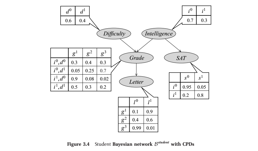 From Ch. 3 of Koller et al. (2009). Here, each row of a CPT gives the distribution over its variable given an assignment of the variable’s parent(s).
According to the rule, any joint assignment of \(\mathcal{X}\) factors as:
\[P_B(I,D,G,S,L) = P_B(I)P_B(D)P_B(G|I,D)P_B(S|I)P_B(L|G)\]So we may calculate an example assignment as:
\[\begin{align} P_B(i^1,d^0,g^2,s^1,l^0) = & \,P_B(i^1)P_B(d^0)P_B(g^2|i^1,d^0)P_B(s^1|i^1)P_B(l^0|g^2)\\ = & \,0.3\cdot 0.6\cdot 0.08\cdot 0.8\cdot0.4 \\ = & \,0.004608\\ \end{align}\]This is to show that a BN along with CPTs gives us a way to calculate probabilities.
Conditional Independence and Bayesian Networks
A Bayesian Network’s utility is in its relation to CI statements:
The BN graph \(\mathcal{G}\), consisting of only nodes and edges, implies a set of CI statements on its accompanying \(P_B\).
This is a consequence of the Chain Rule for calculating probabilities.
Further, we have a not-at-all-obvious fact:
A BN graph represents all \(P\)’s that satisfy its CI statements and each \(P\) could be obtained with an appropriate choice of CPTs.
This is to say, there does not exist a \(P\) with CI statements exactly representable by some \(\mathcal{G}\) whose probabilities can’t be produced by the Chain rule and a choice of CPTs. It eliminates a potential limit on distributions representable as BNs.
For a BN, one way to express its CI statements is as:
\[(X_i \perp\textrm{NonDescendants}_{X_i} \vert \textrm{Pa}_{X_i}^\mathcal{G})\textrm{ for all }X_i \in \mathcal{X}\]So in the student example, it produces:
\[(L\perp I,D,S|G)\\ (S\perp D,G,L|I)\\ (G\perp S|I,D)\\ (I\perp D)\\ (D\perp I,S)\\\]The third statement tells us that if we already know the student’s intelligence and their class’s difficulty, then knowing their SAT score won’t help us guess their grade. This is because the SAT score is correlated with their grade only via their intelligence, which is already known.
These are referred to as the BN’s local semantics. To complicate matters, there are almost always many other CI statements associated with a BN graph outside of the local semantics. To determine those by inspecting the graph, we may use the D-separation algorithm, which won’t be explained here.
To summarize:
Since a BN is a way of representing CI statements and since such statements are required for handling a complex system’s joint distribution, we have good reason to use a BN to represent such a system. Doing so will allow us to answer probability and MAP queries.
It’s worth emphasizing that the decision to represent a system with a particular BN or something else is a delicate and difficult one. The general task of representation is far from settled. Here, at least, we’ve seen computational considerations are strong motivators.
But the representative capacity of BN’s has limits. It’s easy to invent \(P\)’s with CI statements that can’t be represent with a BN. To capture a different class of CI statements, we consider the next type of PGM.
The Markov Network
Like a BN, a Markov Network (‘MN’) is composed of a graph \(\mathcal{H}\) and a probability distribution \(P_M\), but in contrast, the graph’s edges are undirected and it may have cycles. Consequently, a MN represents a different set of CI statements. However, the lack of directionality means we can no longer use CPDs. Instead, this information is delivered with a factor, a function mapping from an assignment of some subset of \(\mathcal{X}\) to a nonnegative number. These factors are used to calculate probabilities with the ‘Gibbs Rule’6.
To understand the Gibbs Rule, we define a complete subgraph. A subgraph is created by selecting a set of nodes from \(\mathcal{H}\) and including all edges from \(\mathcal{H}\) that are between nodes from this set. A complete graph is one which has every edge it can; each node has an edge to every other node. A complete subgraph is also called a clique.
Next, suppose \(\mathcal{H}\) breaks up into \(m\) complete subgraphs7. That is, the union of all nodes and edges across the subgraphs yields all nodes and edges of \(\mathcal{H}\). We’ll write the random variables associated with the nodes of these subgraphs as \(\{\mathbf{D}_i\}_{i=1}^m\). There is one factor, labeled \(\phi_i(\cdot)\), for each subgraph. Each takes an assigment of their respective \(\mathbf{D}_i\) as input. We say the scope of the factor \(\phi_i(\cdot)\) is \(\mathbf{D}_i\). We refer to these factors collectively as \(\Phi\), meaning \(\Phi=\{\phi_i(\mathbf{D}_i)\}_{i=1}^m\).
The Gibbs Rule states a probability is calculated as8:
\[P_M(X_1,\cdots,X_n) = \frac{1}{Z} \prod_{i=1}^m \phi_i(\mathbf{D}_i)\]where \(Z\) is the normalizer ensuring probabilities sum to one over the domain of \(\mathcal{X}\):
\[Z = \sum_{\mathbf{x}\in \textrm{Val}(\mathcal{X})} \prod_{i=1}^m \phi_i(\mathbf{D}_i)\]
The CI statements represented with a MN are considerably easier to infer than in the case of a BN:
A MN implies the CI statement (\(\mathbf{X} \perp \mathbf{Y} \vert \mathbf{Z}\)) if all paths between \(\mathbf{X}\) and \(\mathbf{Y}\) go through \(\mathbf{Z}\).
To illustrate, below is a MN for the system \(\mathcal{X}=\{A,B,C,D\}\) and the CI statements it represents:
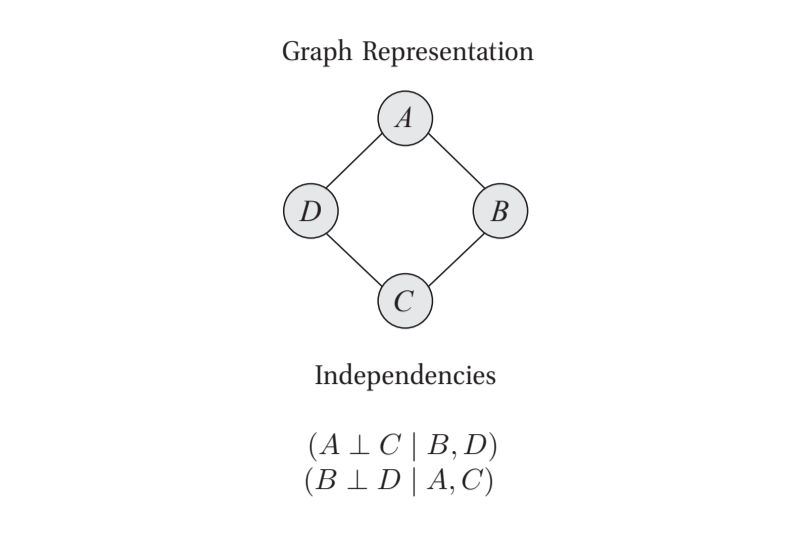 From figure 1.1 from Koller et al. (2009)
As is clear, it’s simple to write the CI statements by inspecting the graph.
With this example, we’ll write the Gibbs Rule computation. We can identify the complete subgraphs as: \(\{\{A,B\},\{B,C\},\{C,D\},\{D,A\}\}\), and so we calculate a probability as:
\[P(A,B,C,D) = \frac{1}{Z}\phi_1(A,B)\phi_2(B,C)\phi_3(C,D)\phi_4(D,A)\]where
\[Z = \sum_{\mathbf{x}\in \textrm{Val}(\mathcal{X})}\phi_1(A,B)\phi_2(B,C)\phi_3(C,D)\phi_4(D,A)\]To repeat, each \(\phi_i(\cdot,\cdot)\) is a function that maps from its given assignment to some nonnegative number. If \(A\) and \(B\) could only take on two values each, \(\phi_1(\cdot,\cdot)\) would relate the four possible assignments to four nonnegative numbers. These functions serve as parameters just as the CPDs did for BNs. Setting these functions brings us from a family of \(P\)’s to a specific \(P\).
But there’s a wrinkle. In the BN case, we said: “A BN graph represents all \(P\)’s that satisfy its CI statements and each \(P\) could be obtained with an appropriate choice of CPDs.”
The analogous statement is not true in the case of MNs. There may exist a \(P\) that satisfies the CI statements of a MN graph, but its probabilities cannot be computed with the Gibbs Rule. Fortunately, these \(P\)’s fall into a simple-but-large category–those which assign a zero probability to at least one assignment. This leads to the following:
Hammersley-Clifford theorem: If \(P\) is such that \(P(\mathbf{X}=\mathbf{x})>0\) for all \(\mathbf{x} \in \textrm{Val}(\mathcal{X})\) –that is, it is a positive distribution– and satisfies the CI statements of \(\mathcal{H}\), then the Gibbs Rule can yield the probabilities of \(P\) with an appropriate choice of factors.9
Comparison of Bayesian Networks and Markov Networks
At this point, we’re not educated enough for a full comparison, so we’ll do a partial one.
First, it’s easier to determine CI statements in a MN; something like the D-separation algorithm isn’t required. This follows from their symmetric undirected edges, which make them natural candidates for some problems. Broadly, MNs do better when we have decidedly associative observations, like pixels on a screen or concurrent sounds. BNs are better suited when the random variables represent components of some causal or sequential structure. Timestamps and domain knowledge are helpful in such a case.
Second, there’s a certain equivalence between MNs and BNs that’ll unify the discussion in subsequent posts:
The probabilities produced by the Chain Rule of any BN can be exactly reproduced by the Gibbs Rule of a specially defined MN.
To see this, we recognize \(P_B(X_i \vert \textrm{Pa}_{X_i}^\mathcal{G})\) within the Chain Rule could be expressed as a factor with \(\mathbf{D}_i=\{X_i\}\cup\textrm{Pa}_{X_i}^\mathcal{G}\), in which case the Chain Rule and the Gibbs Rule are equivalent. This means any theorems regarding the Gibbs Rule also apply to the Chain Rule.
What this does not mean is that MNs are a substitute for BNs. Their equivalence in this regard does not imply their equivalence in all regards and so they are of different utility in different circumstances.
Third, we’ll see parameter learning and structure learning are notably harder for Markov Networks. As mentioned in chapter 2 of Jordan (2003), the difficulty can be traced to BNs’ explicit notion of local probabilities, whereas MNs have locality more generally defined. By locality, we mean small subsets of variables varying together to produce global variations when linked. For a BN, locality is expressed with conditional probabilities, whereas for a MN, it’s expressed with unnormalized quantifications of agreement. For a BN, normalization (to ensure probabilities sum to one) happens at the level of an individual \(X_i\) when constructing its CPT. For a MN, normalization involves integration over the exponentially large domain of \(\mathcal{X}\). This can make MNs much more computationally burdensome.
But differences aren’t only computational. For example, a BN’s conditional probabilities enable ancestral sampling, where samples of \(\mathcal{X}\) can be generated one variable at a time. This involves ordering variables according to \(\mathcal{G}\)’s topological ordering, where each comes before their respective parents. The first variables are sampled unconditionally, which provides parent assignments for sampling subsequent variables per their CPTs, until all variables are sampled. For a MN, no notion of local probability is defined, so no analogous sampling method is available. Instead, we have to refer to more exotic methods, like those discussed in Part 4.
For an in depth comparison, see Domke et al. (2008).
The Next Step
Suppose we’ve determined a graphical model along with its parameters. How do we answer probability queries? This can be answered three seperate ways:
References
-
D. Koller and N. Friedman. Probabilistic Graphical Models: Principles and Techniques. MIT Press. 2009.
-
M. I. Jordan. An Introduction to Probabilistic Graphical Models. University of California, Berkeley. 2003.
-
K. Murphy. Machine Learning: A Probabilistic Perspective. MIT Press. 2012.
-
M. Wainwright and M. I. Jordan. Graphical Models, Exponential Families, and Variational Inference. Foundations and Trends in Machine Learning. 2008.
-
S. Kotiang, A. Eslami. A probabilistic graphical model for system-wide analysis of gene regulatory networks. Bioinformatics, Volume 36, Issue 10, Pages 3192–3199. 2020.
-
A. Farasat, A. Nikolaev, S. N. Srihari and R. H. Blair. Probabilistic graphical models in modern social network analysis. Social Network Analysis and Mining. 2015.
-
J. Domke, A. Karapurkar, and Y. Aloimonos. Who Killed the Directed Model? CVPR. 2008
Something to Add?
If you see an error, egregious omission, something confusing or something worth adding, please email dj@truetheta.io with your suggestion. If it’s substantive, you’ll be credited. Thank you in advance!
Footnotes
-
A collection of applications can be found here and section 2.4 of Wainwright et al. (2008) describes classic uses in detail. ↩
-
I wrote about the causal graphical model work we did at Lyft with two blogs: Causal Forecasting at Lyft (Part 1) and Causal Forecasting at Lyft (Part 2) ↩
-
In fact, this isn’t the fully general problem specification. In complete generality, the set of random variables may grow or shrink over time. ↩
-
This is the one exception where we don’t refer to a set of random variables with a bold uppercase letter. ↩
-
If \(X_i\) doesn’t have any parents, the CPD is the unconditional probability distribution of \(X_i\). ↩
-
‘Gibb’s Rule’ isn’t a real name I’m aware of, but the form of the distribution makes it a Gibbs distribution and I’d like to maintain an analogy to BNs, which has the Chain Rule. ↩
-
As pointed out on pages 9-10 of Wainwright et al. (2008), one could specify the cliques as maximal without loss of generality, but there are computational reasons to consider non-maximal cliques. ↩
-
It’s hidden from this notation, but we’re assuming it’s clear how to match up the assignment of \(X_1,\cdots,X_n\) with the assignments of the \(\mathbf{D}_i\)’s. ↩
-
The implication goes the other way as well: If the probabilities of \(P\) can be calculated with the Gibbs Rule, then it’s a positive distribution which satisfies CI statements implied by a graph which has complete subgraphs of random variables that correspond to the random variables of each factor. This direction, however, doesn’t fit into the story I’m telling, so it sits as a footnote. ↩