The Fundamental Law of Active Management
Posted: Updated:
The Fundamental Law of Active Management is a way of viewing risk adjusted returns, arguably the most important measure of an investment strategy, in terms of two core components. A performant strategy must do well at one or both. Crucially, knowledge of the components guides decisions for improving performance. In fact, once understood, it’s natural to judge all strategies in this manner.
Additionally, the law governs hundreds of billions of investment dollars. It was asserted and substantiated in the 1999 book Active Portfolio Management by Richard Grinold and Ronald Kahn. Notably, Kahn has been the head of equity research at BlackRock for over two decades. From the few folks I know at BlackRock, many of their multi-billion dollar strategies are framed by the ideas presented in this book.
In this post, we’ll cover the law in a reduced form, without reference to market returns, betas, alphas, and the like. For easy digestion, we’ll see the law operating in a simple, idealized game. Nevertheless, the essential features and its relevance to the reality of investing will be made clear.
The Game
A player is faced with five correlated bets, each normally distributed with a mean of zero. A sample of them may be pictured as vertical lines:
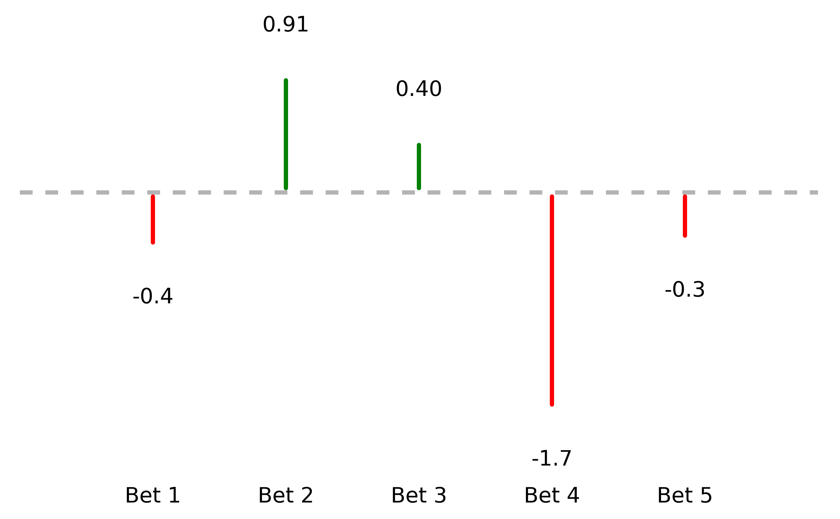 A player faces five correlated bets. Their outcomes may be visualized as vertical lines.
We’ll label this random vector as \(\mathbf{y}\).
The player must pick a number for each bet, called the holding, before seeing the bet outcomes. Their goal is to select holdings such that its sum-product with bet outcomes is highest. If we imagine each holding as a horizontal line starting at the base of the outcome line and suppose each holding is one, we can picture the product as the sum of the colored area:
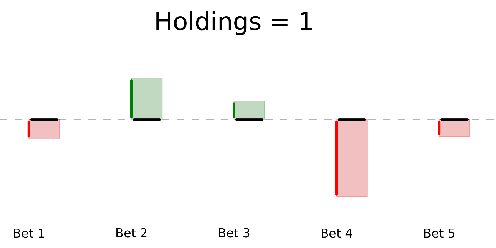 The holdings interact with outcomes as the total area, where red is considered a negative area.
As we’ll formalize later, the goal is to maximize the green area less the red area and to do so with high probability. This is a precise analogy to an investor’s objective of maximizing return while minimizing risk.
If \(\mathbf{h}\) is a vector of holdings, \(\mathbf{h}^{\top}\mathbf{y}\) is the green area less the red area. We’ll refer to this as the player’s winnings.
As the game is currently presented, there is nothing the player can do to improve winnings; any choice of \(\mathbf{h}\) yields the same zero-expected-value of \(\mathbf{h}^{\top}\mathbf{y}\). To move beyond this, we assume before each bet, the player receives gaussian signals correlated with the bet outcomes:
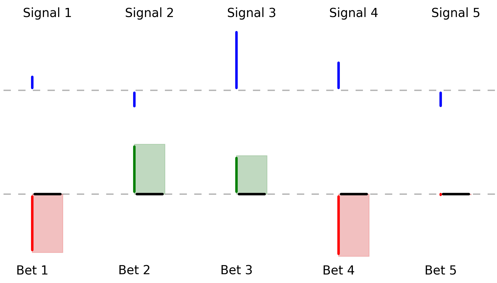 Before forming holdings, a player may observe signals correlated with the bet outcomes.
Let \(\mathbf{z}\) be the random vector of signals.
Still, more information is needed, as the relation between the signal and bet outcomes needs to be understood. We assume the following is known:
- \(\textrm{var}(\mathbf{y})\) : the \(5\)-by-\(5\) covariance matrix of the bet outcomes. Considering the bet outcomes are normally distributed with a mean of zero, this fully dictates their distribution prior to an observation of \(\mathbf{z}\).
- \(\textrm{cov}(\mathbf{z},\mathbf{y})\) : a \(5\)-by-\(5\) cross-covariance matrix specifying covariances between each bet outcome and each signal.
- \(\textrm{var}(\mathbf{z})\) : a \(5\)-by-\(5\) covariance matrix of the signals.
We now have enough information to form performant holdings.
What is the optimal player strategy?
A desireable strategy must have two characteristics:
- A high expected return
- A low variance
These, following an observation of \(\mathbf{z}\), may be measured and balanced as a function of \(\mathbf{h}\) with the following utility function:
\[U(\mathbf{h} \vert \mathbf{z}) = \mathbb{E}[\mathbf{h}^{\top} \mathbf{y} \vert \mathbf{z}] - \lambda \textrm{var}(\mathbf{h}^{\top} \mathbf{y} \vert \mathbf{z})\]where:
- \(\mathbb{E}[\mathbf{h}^{\top} \mathbf{y} \vert \mathbf{z}]\) is the expected sum of areas conditional on an observation of \(\mathbf{z}\). In the investor reality, these are expected (excess) returns.
- \(\textrm{var}(\mathbf{h}^{\top} \mathbf{y} \vert \mathbf{z})\) is the variance of the sum of areas conditional on an observation of \(\mathbf{z}\). In the investor reality, this is risk.
- \(\lambda\) represents the player’s risk aversion; it’s a positive value characterizing their preference for trading off expected return with risk. For example, \(\lambda=2\) implies a reduction of one unit of variance is worth an increase of two units in expected return.
The expression may be written:
\[U(\mathbf{h} \vert \mathbf{z}) = \mathbf{h}^{\top} \mathbb{E}[\mathbf{y} \vert \mathbf{z}] - \lambda \mathbf{h}^{\top} \textrm{var}(\mathbf{y} \vert \mathbf{z})\mathbf{h}\]As \(U(\mathbf{h} \vert \mathbf{z})\) is to be optimized with respect to \(\mathbf{h}\), we may do so starting with the gradient:
\[\frac{d}{d \mathbf{h}} U(\mathbf{h} \vert \mathbf{z})= \mathbb{E}[\mathbf{y} \vert \mathbf{z}] - 2\lambda \textrm{var}(\mathbf{y} \vert \mathbf{z})\mathbf{h}\]Setting this to zero yields an expression for the optimal holdings:
\[\mathbf{h}_{opt} = \frac{1}{2\lambda}\textrm{var}(\mathbf{y} \vert \mathbf{z})^{-1}\mathbb{E}[\mathbf{y} \vert \mathbf{z}]\]What remains is to express \(\textrm{var}(\mathbf{y} \vert \mathbf{z})\) and \(\mathbb{E}[\mathbf{y} \vert \mathbf{z}]\) as a function of what is known. To this end, we are aided by well known results of the multivariate normal distribution:
\[\begin{align} \mathbb{E}[\mathbf{y} \vert \mathbf{z}] = & \,\mathbb{E}[\mathbf{y}] + \textrm{cov}(\mathbf{y},\mathbf{z})\textrm{var}(\mathbf{z})^{-1}(z-\mathbb{E}[\mathbf{z}])\\ = & \,\textrm{cov}(\mathbf{y},\mathbf{z})\textrm{var}(\mathbf{z})^{-1}(z-\mathbb{E}[\mathbf{z}])\\ \phantom{=} & \\ \textrm{var}(\mathbf{y} \vert \mathbf{z}) = & \,\textrm{var}(\mathbf{y}) - \textrm{cov}(\mathbf{y},\mathbf{z}) \textrm{var}(\mathbf{z})^{-1} \textrm{cov}(\mathbf{z},\mathbf{y})\\ \end{align}\]Given an observation of the signal, a player’s risk aversion \(\lambda\), and the assumed-to-be-known distributional information from the previous section, we can construct the player’s optimal holdings as:
\[\mathbf{h}_{opt} = \frac{1}{2\lambda}\Big(\textrm{var}(\mathbf{y}) - \textrm{cov}(\mathbf{y},\mathbf{z}) \textrm{var}(\mathbf{z})^{-1} \textrm{cov}(\mathbf{z},\mathbf{y})\Big)^{-1}\textrm{cov}(\mathbf{y},\mathbf{z})\textrm{var}(\mathbf{z})^{-1}(z-\mathbb{E}[\mathbf{z}])\]Playing the Game
Using the optimal strategy and playing the game fifteen times gives us:
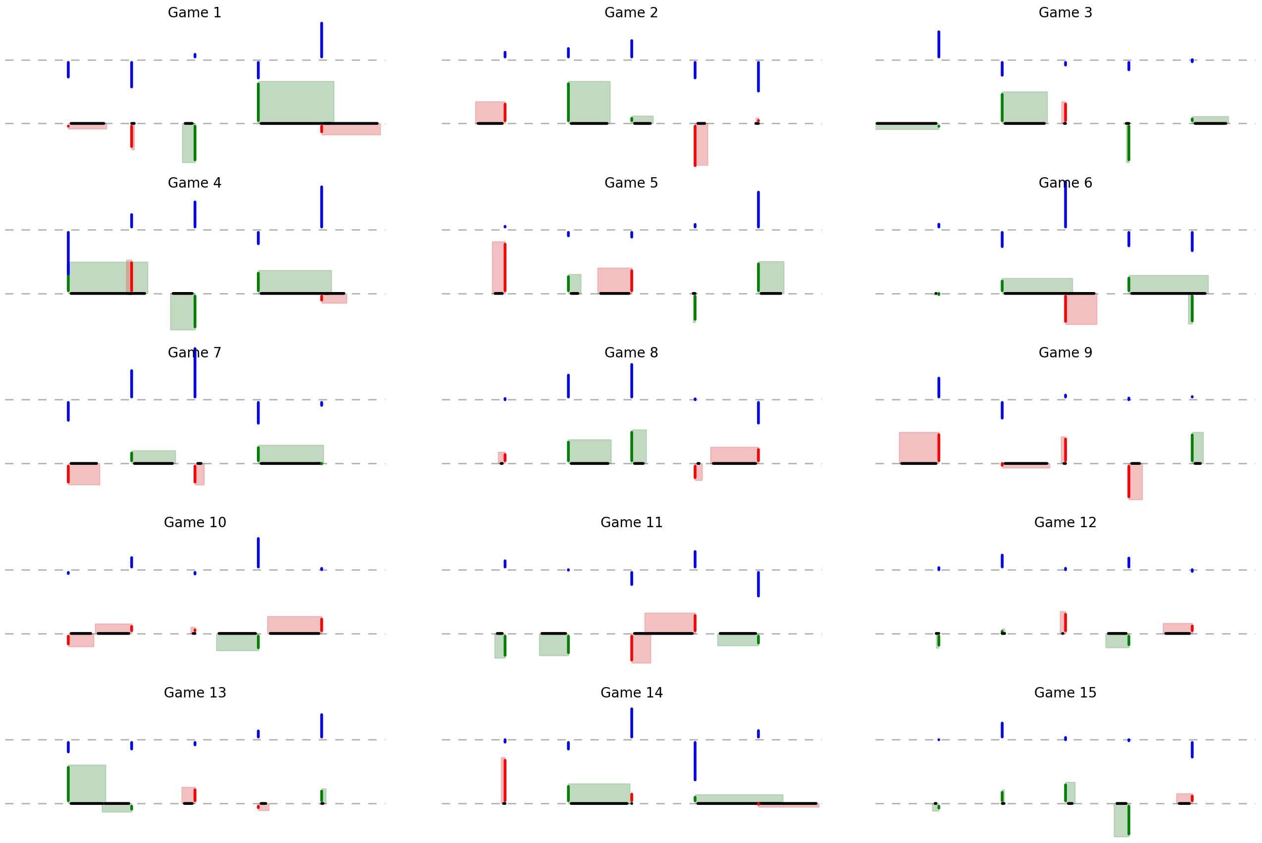 Many plays of the game using the optimal strategy.
By an eye ball evaluation, there’s more green than red, indicating the strategy works.
Naturally, we ask: What is the distribution of winnings? If we run 10,000 games, we observe the following histogram:
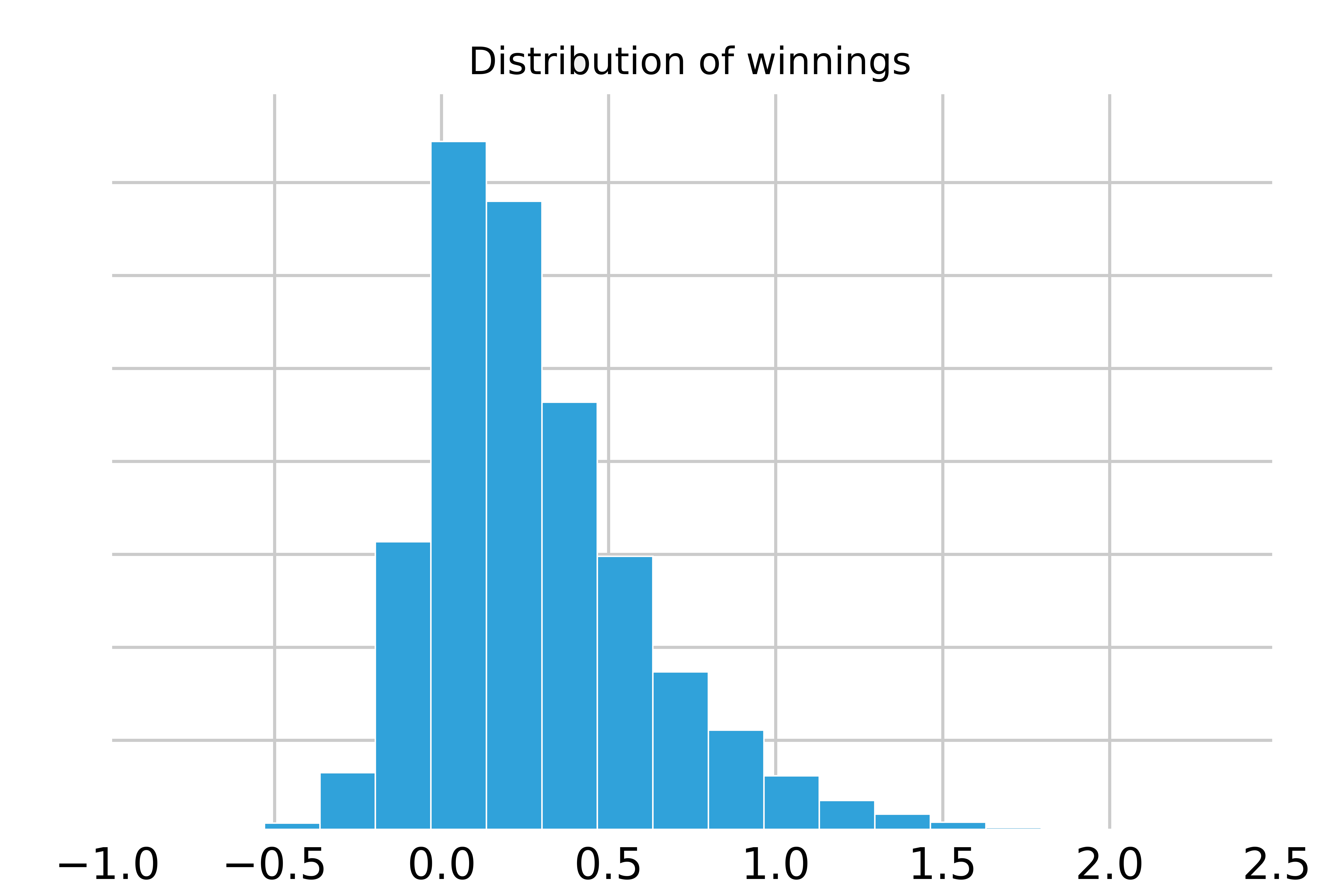
This histogram represents all that we care about when implementing the optimal strategy for a given game. It is the full distribution of outcomes, inclusive of both the expected return and risk. This will be important to recall after we consider the following scenario.
Choosing a Game
Imagine we are exploring games being played optimally. We will inspect the distributions of winnings for each game and pick the most attractive one. How should we select the game?
There is in fact a correct answer.
We should choose the game with the highest Information Ratio1 (‘IR’):
\[\textrm{IR}_g = \frac{\mu_g}{\sigma_g}\]where \(\mu_g\) is the expected winnings and \(\sigma_g\) is the standard deviation of winnings for game \(g\).
If we select the game with the highest IR, we’ll select that which yields the highest expected utility, which represents the best risk adjusted return.
In short, IR captures everything that makes a game attractive according to \(U(\mathbf{h} \vert \mathbf{z})\). What’s notable is the choice does not depend on the risk aversion parameter \(\lambda\). Regardless of whether \(\lambda\) is 2 or 20, a player always prefers a game where a small amount of risk trades for a large return.
For insight, imagine a plot with \(\mu\) along the vertical axis and \(\sigma\) along the horizontal. Within this space, we can draw curves of constant utility:
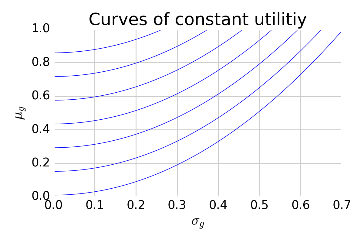 This shows curves of constant utility, where higher utility is realized towards the upper left. These curves are curved because the horizontal axis represents standard deviation whereas the utility function considers variance.
In this space, we may show the region of risk-reward profiles achievable by an \(\mathbf{h}\)-forming strategy. For a given game, it looks like:
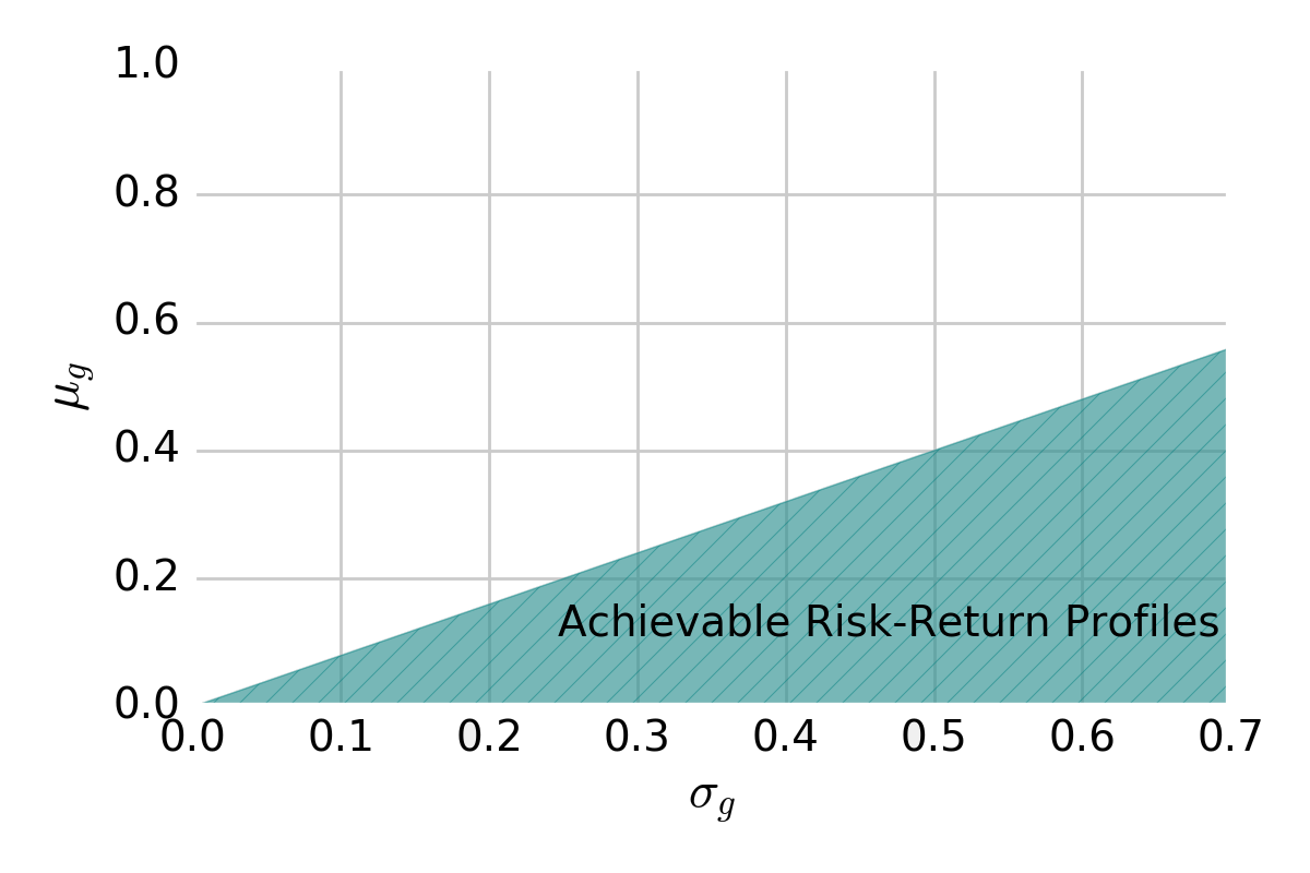 Region of risk-return combinations achievable with an \(\mathbf{h}\)-forming strategy
When overlaying curves of constant utility and maximizing utility with an \(\mathbf{h}\)-forming strategy, we pick the point tangent to the slope of the line that separates the achievable from the unachievable:
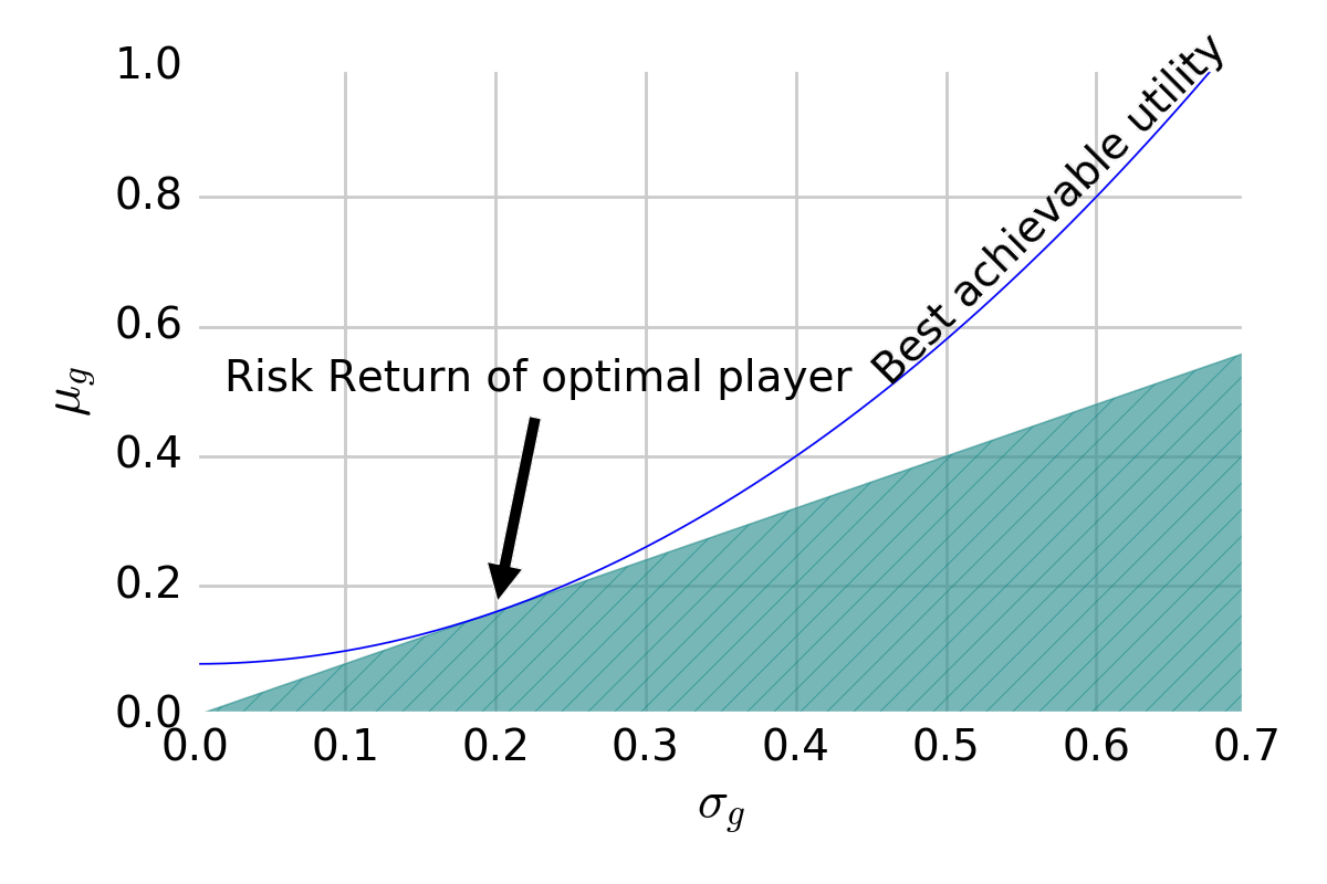
This point dictates the expected return and standard deviation of the winnings of the optimal strategy. Crucially, games can be ranked by this point’s utility by ranking games by IR under optimal play.
Decomposing IR
By this point, we’ve yet to reveal the two core components of an investment strategy, mentioned at the beginning. Those components are seen with the following decomposition.
IR has a simple, approximate-yet-accurate decomposition that defines the Fundamental Law:
\[\textrm{IR} \approx \textrm{IC}\sqrt{\textrm{BR}}\]where:
- Information coefficient (IC): average measure of correlation between \(\mathbf{z}\) and \(\mathbf{y}\)
- Breadth (BR): number of independent bets
This defines, in simplest terms, what makes a game attractive. In general, think ‘doubling IC is worth quadrupling the number of bets.’
For intuition, consider a simple case. Say \(\mathbf{y}\) has length 10 and is uncorrelated with itself and this is similarly true for \(\mathbf{z}\). On average, an element of \(\mathbf{z}\) has a correlation of \(0.05\) with an element of \(\mathbf{y}\). In this case, \(\textrm{IR} = 10\times0.05 = 0.5\). That is, the best we can hope for is \(0.5\) in expected return for every unit of standard deviation tolerated.
Back to the Investor’s Reality
To conclude, we’ll relate this game-playing with the reality of investing.
As has been alluded to, the game is an investment strategy. The holdings are holdings in financial assets. The rectangular areas are excess returns realized on those assets. We decide those holdings with some signal, at least implicitly, that has some correlation with the performance of those financial assets. This is true of any excess-return-seeking strategy; at some level, it must exploit correlations across time.
Investors are like players. They invest in some strategy (or ‘play a game’) with some leverage dictated by their risk aversion. That is, they exploit the game to its best achievable risk-return profile, ramping up the return until they reach their maximum tolerance of risk2.
When evaluating performance, we must consider a risk-adjusted return metric, like IR, to summarize perform independently of risk appetite. By this metric and from the above, we can deduce:
An investment strategy is attractive if it:
- involves strong correlations between signals and returns.
- uses signals that are weakly or not correlated with themselves.
- uses returns that are weakly or not correlated with themselves.
- takes a large number of bets.
Such qualities can be useful when judging strategies. For example, consider strategies involving the following signals:
- a 0.2 correlated indicator to proxy biotech earning reports before publication.
- a 0.01 correlated indicator to proxy the difference between opening and closing prices of US Equities.
Without knowledge of the law, the first signal appears more attractive. A .2 correlated signal is extremely strong. But it is in fact less valuable than the second signal, since there are thousands of times more opportunities to bet on it. We can bet on it every day and across every US equity, whereas the first applies to a particular sector and can only be exploited several times a year.
In summary:
According to a standard utility function, the Information Ratio fully captures the appeal of an investment strategy. The Fundamental Law of Active Management reveals this quality as approximately the product of the Information Coefficient and the square root of the Breadth. Therefore, performant strategies will frequently (high BR) trade with signals which strongly correlate (high IC) with future returns.
A Word of Caution
It is important to recognize what is being stated with the Fundamental Law. It regards the case where certain distributional information is known. That is, we assume we know things like \(\textrm{cov}(\mathbf{z},\mathbf{y})\). In reality, these must be estimated, incurring errors that seriously complicate the above reasoning. At the least, we no longer can speak of a strategy’s IR as though it’s observed. Rather, we’d need to consider the distribution of probable values, burdening us with an additional and challenging dimension of uncertainty.
References
-
Grinold, R. and R. Kahn, Active Portfolio Management: A Quantitative Approach for Providing Superior Returns and Controlling Risk. 2nd ed. New York: McGraw-Hill. 1999.
-
R. Clarke, H. deSilva, and S. Thorley. The Fundamental Law of Active Portfolio Management. Journal of Investment Management, 2006.
Something to Add?
If you see an error, egregious omission, something confusing or something worth adding, please email dj@truetheta.io with your suggestion. If it’s substantive, you’ll be credited. Thank you in advance!
Footnotes
-
The information ratio, in general, is defined with respect to a benchmark, but I’m intentionally leaving that out. In my humble opinion, in this context, it complicates the math more so than necessary. ↩
-
It’s definitely an assumption that investors are risk-return utility maximizers. But we ultimately have to assume something about how people act on their risk appetite, so this seems reasonable. ↩