The Fisher Information
Posted: Updated:
To understand the Fisher Information, we’ll start with its goal, proceed with intuitive geometry and arrive at its definition. To broaden the applicability, we’ll discuss its generalization to higher dimensions. At that point, we’ll be unexpectedly close to a major theorem in statistics, so we’ll cover that as well.
The Goal of the Fisher Information
Suppose a scalar random variable \(X\) and an unknown parameter \(\theta\) are related with some known density function:
\[p(X \vert \theta)\]The Fisher Information answers the question:
How useful is \(X\) in determining \(\theta\)?
Intuitively, \(X\) contains a large amount of information regarding \(\theta\) if an observation1 of \(X\) precisely locates \(\theta\). In fact, we’ll use this as our definition of information.
For intuition, what behavior would characterize opposite extremes? Consider the likelihood function, \(\log p(x_i \vert \theta)\), in two circumstances, where \(X\) is either very informative or uninformative regarding the location of \(\theta\):
- Informative: \(X\) is normally distributed with a known and small \(\sigma^2\) of \(1\). The mean \(\mu\) is the unknown \(\theta\). This gives us enough information to write \(p(X \vert \theta)\).
- Uninformative: \(X\) is the same as before, except we use a relatively large \(\sigma^2\) of \(25\).
Next, we’ll generate samples, the \(x_i\)’s, using the true mean of 5 and plot the \(\log p(x_i \vert \theta)\)’s vs \(\theta\):
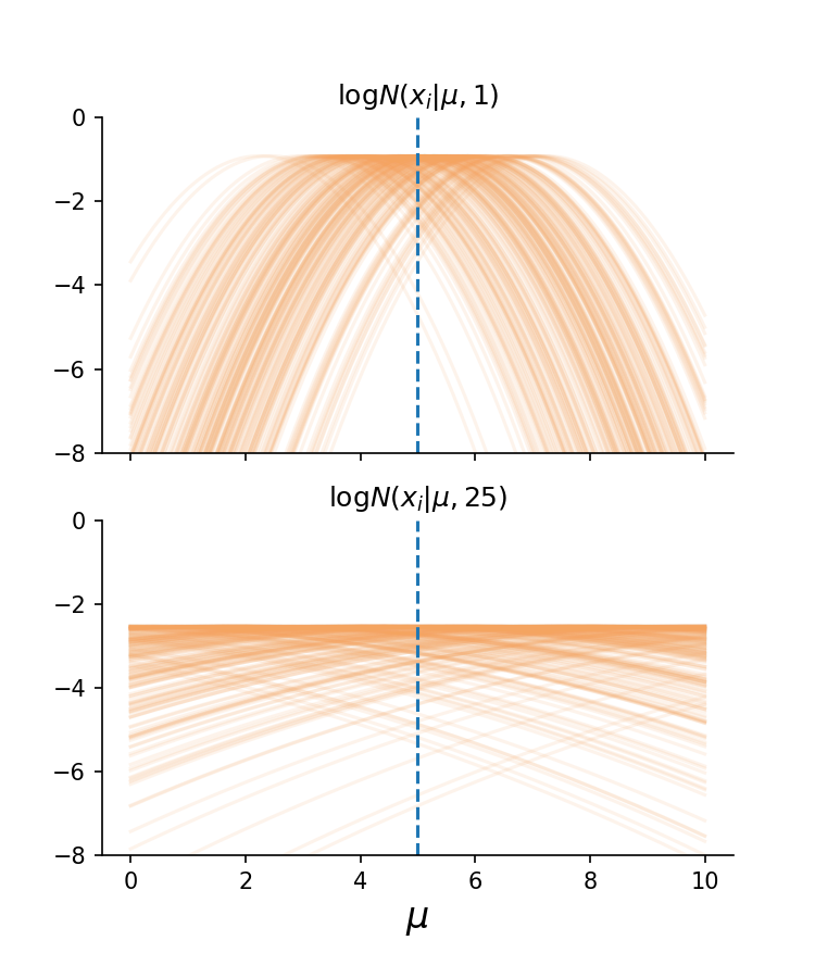 The top plot shows different log likelihood curves for different samples of \(X\). Their peaks concentrate tightly around the true parameter value. \(\\\)The below plot is similar, except it comes from a distribution with a larger variance and so, the true parameter value is less well identified.
In which circumstance is it easier to locate the true mean? Isn’t it obvious?
In effect, each curve is providing their own vote – their peak – of the true parameter’s location. When these curves have tighter peaks, thereby restricting the range of possible \(\mu\) values that could explain all such peaks, we say \(X\) is informative for \(\mu\) (or more generally, \(\theta\)).
How is information measured?
It’s done by looking at the slopes of the curves above, which are called score functions:
\[\textrm{score}_i(\theta) = \frac{\partial}{\partial \theta} \log p(x_i \vert \theta)\]To see the mechanics, we plot the derivative functions below one of the previous graphs. We pick a few \(\mu\) values and evaluate slopes for those values, yielding a set of numbers for each. For each set, we plot their histogram:
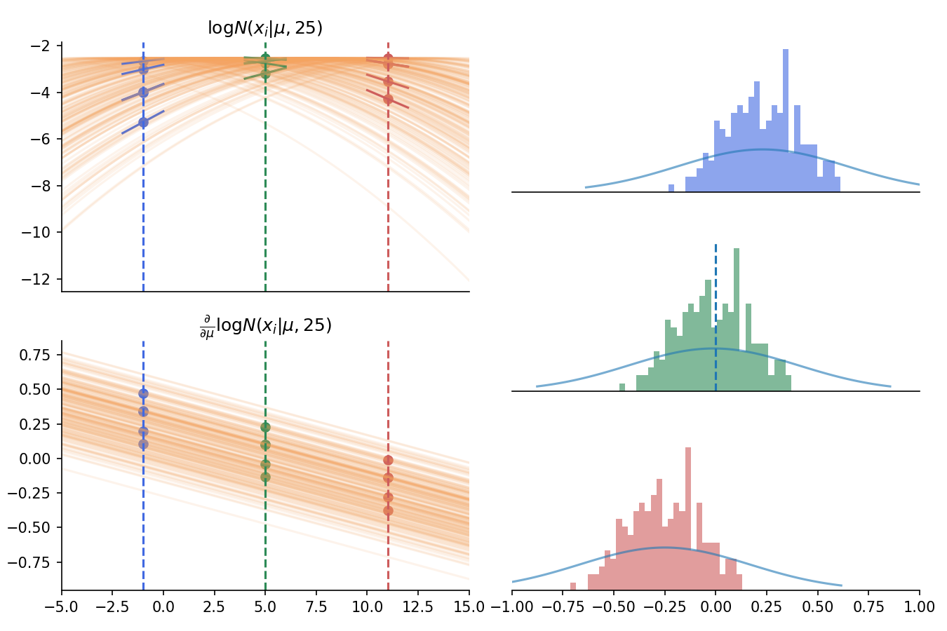 Left: the log likelihoods as a function of \(\mu\) across many \(X\) samples, with their derivative functions plotted below \(\\\) Right: histograms of slopes for different choices of \(\mu\). Notice the middle histogram has a mean of zero when it’s evaluated at the true value of \(\mu\).
Imagine we squeeze the top left curves such that they become more peaked and, as explained, \(X\) becomes more informative. What would happen?
As the curves become more peaked, the slopes at an evaluation point vary more widely. That is, the histograms on the right become wider. Mechanically, we’re encountering the fact:
We’re more likely to come across extreme derivatives when we’re dealing with highly peaked log likelihoods.
This is the key insight of the Fisher Information.
But before moving forward, there’s an important observation that generalizes nicely. That is, when the evaluation point for \(\mu\) is the true \(\mu\) (5 in the case), the mean of the slopes is zero. We can see this in the middle histogram above. This may be written in its general form2:
\[\mathbb{E}_{\theta^*}[\frac{\partial}{\partial\theta}\log p(X \vert \theta) \big|_{\theta=\theta^*}] = 0\]With this, we may describe the Fisher Information. It’s a function of a parameter that gives the variance of the middle histogram:
\[\mathcal{I}(\theta^*) = \textrm{var}_{\theta^*}(\frac{\partial}{\partial\theta}\log p(X \vert \theta) \big|_{\theta=\theta^*})\]One thing worth clarifying is the two roles \(\theta^*\) is playing. It is both the assumed true parameter value and the evaluation point for the derivative3.
Next, because that expectation is zero, it simplifies further:
\[\mathcal{I}(\theta^*) = \mathbb{E}_{\theta^*}\big[\big(\frac{\partial}{\partial\theta}\log p(X \vert \theta) \big|_{\theta=\theta^*}\big)^2\big]\]It turns out if \(\log p(X \vert \theta)\) is twice differentiable, then:
\[\mathbb{E}\big[\big(\frac{\partial}{\partial\theta}\log p(X \vert \theta) \big|_{\theta=\theta^*}\big)^2\big] = -\mathbb{E}\big[\frac{\partial^2}{\partial\theta^2}\log p(X \vert \theta) \big|_{\theta=\theta^*}\big]\]This isn’t obvious, but not wholly unreasonable either. We expect a wide variance in the derivatives if they are changing extremely at that point. Derivatives that are changing extremely have a high absolute derivative themselves; they reflect a high second derivative.
The Multidimensional Fisher Information
The multidimensional case is a fairly seamless generalization of the 1D case.
To do so, we’ll carefully consider our actions in the 1D case. The Fisher Information accepts one parameter value and returns a single number, a number which describes the distribution of the log-likelihood derivatives. So in the \(D\)-dimensional case, the Fisher Information should accept a length-\(D\) parameter vector and return something that describes the distribution of the gradient, the multidimensional analog of a derivative. The gradient is a vector, so we should think: ‘variance is to a scalar as a (something) is to a vector.’
What fits perfectly is the covariance matrix. The Fisher Information will accept a parameter vector and return a covariance matrix that describes the distribution of the log likelihood gradient. This leads us to:
\[\mathcal{I}(\boldsymbol{\theta}^*)_{i,j} = \mathbb{E}_{\boldsymbol{\theta}^*}\big[\big(\frac{\partial}{\partial\theta_i}\log p(X \vert \boldsymbol{\theta}) \big|_{\boldsymbol{\theta}=\boldsymbol{\theta}^*}\big)\big(\frac{\partial}{\partial\theta_j}\log p(X \vert \boldsymbol{\theta}) \big|_{\boldsymbol{\theta}=\boldsymbol{\theta}^*}\big)\big]\]\(\mathcal{I}(\boldsymbol{\theta}^*)\) is the full covariance matrix. The element in the \(i\)-th row and \(j\)-th column is the expected product of the \(i\)-th and \(j\)-th elements of the gradient. Since each of these will have an expectation of zero separately, their expected product is also their covariance.
Also, we get a similar second derivative simplification as we saw earlier:
\[\mathcal{I}(\boldsymbol{\theta}^*)_{i,j} = -\mathbb{E}_{\boldsymbol{\theta}^*}\big[\frac{\partial^2}{\partial\theta_i\partial\theta_j}\log p(X \vert \boldsymbol{\theta}) \big|_{\boldsymbol{\theta}=\boldsymbol{\theta}^*}\big]\]Here, we recognize the Hessian matrix in this expression, which is just a multidimensional analog of the second derivative.
In words:
The covariance matrix of the log likelihood’s gradient evaluated at the given parameter values and according to the distribution dictated by the those values is the negative expected Hessian matrix of the log likelihood.
Multidimensional Intuition
Imagine generalizing the earlier example to the two-parameter case; so we consider both the mean and the variance parameters, but our random variable is still a scalar. The sampled score functions would no longer be 1D curves but 2D domes. The histograms on the right would be 2D histograms. A very spread out histogram would imply we could locate the true parameter vector quite well.
A very spiked histogram would imply we often see very similar gradients and the lack of diverse information makes it hard to nail down the true parameters.
But we can take it a little further. A 2D histogram can be very spread out in one direction and very thin in the orthogonal direction. Our reasoning extrapolates well here. The spread out direction is the direction along which we can easily separate true from not-true parameters. Along the thin direction, we can’t make such a separation.
(If this explanation isn’t making it click, you can see it animated in my video on the topic.)
The Distribution of the MLE Estimate
There’s a major theorem that’s quite easy to state from here. Suppose we sample \(N\) IID random variables. Then the Maximum Likelihood Estimate (MLE) of \(\boldsymbol{\theta}^*\) will come from a distribution that is asymptotically normal:
\[\boldsymbol{\theta}_{MLE} \sim \mathcal{N}(\boldsymbol{\theta^*},\frac{1}{N}\mathcal{I}(\boldsymbol{\theta^*})^{-1})\]as \(N \rightarrow \infty\). Since \(\boldsymbol{\theta}^*\) cannot be known, a typical concession is to use \(\boldsymbol{\theta}^*=\boldsymbol{\theta}_{MLE}\).
One remarkable consequence is:
In much the same way we may use the Central Limit Theorem for hypothesis testing, we may use this to do the same in the multivariable case.
A Clarification
This explanation is dangerously close to the question:
What is the distribution of the unknown parameter?
This question isn’t answered here and is much better addressed with bayesian methods. The Fisher Information is a frequentist concept, where we assume the true parameter has a fixed value. To a frequentist, the question doesn’t make sense. To them, only random variables have distributions and the true parameter is no such thing.
References
I first read of the Fisher Information in Hastie et al. (2009) a long time ago. A. Ly et al. (2017) was the deep dive source I used mostly for this post.
-
A. Ly, M. Marsman, J. Verhagen, R. Grasman and E. Wagenmakers. A Tutorial on Fisher Information. University of Amsterdam 2017
-
T. Hastie, R. Tibshirani and J. H. Friedman. The Elements of Statistical Learning: Data Mining, Inference, and Prediction 2nd ed. New York: Springer. 2009.
Something to Add?
If you see an error, egregious omission, something confusing or something worth adding, please email dj@truetheta.io with your suggestion. If it’s substantive, you’ll be credited. Thank you in advance!
Footnotes
-
Yes, ‘an’ observation. The Fisher Information is a measure of a random variable itself, not some set of observations. However, when it’s used to determine convergence properties of \(N\) observations, it’s typical to treat this as single observations from \(N\) IID random variables. Therefore, if we speak about observations, the singular count is most appropriate. ↩
-
The subscript \(\theta^*\) next to the expectation sign means the expectation is according to the distributed per \(\theta^*\). ↩
-
If you’re bothered by this, you’re probably a Bayesian. If the Fisher Information is telling us our ability to locate the true parameter, shouldn’t it not rely on knowing the true parameter? Yes, indeed. Frequentist statistics is odd. ↩