Bias-Variance Trade-Off
Posted: Updated:
The bias-variance trade-off relates to the bias-variance decomposition, a precious insight into the challenge of generalization:
Generalization: How can one create a model from a sample of data that’ll predict well on another, unseen sample of data?
To understand the insight, we start with the assumptions.
Assumptions
We assume \(y\) and the vector \(\mathbf{x}\) are related with some unknown true function \(f(\cdot)\) as:
\[y = f(\mathbf{x}) + \epsilon\]where \(\epsilon\) is irreducible noise born from an error distribution where \(\mathbb{E}[\epsilon]=0\) and \(\textrm{var}(\epsilon)=\sigma_{\epsilon}^2\). In words, we assume an observed \(y_0\) is generated by plugging the associated \(\mathbf{x}_0\) into \(f(\cdot)\) and adding an \(\epsilon_0\) sampled from the error distribution.
In general, the goal is to infer \(f(\cdot)\) from data. We’ll label the estimated function as \(f_{\textrm{est}}(\cdot)\) and we’ll call the algorithm that ingests training data to produce it the ‘estimating procedure’.
Next, it’ll help to consider a theoretical environment where we can repeatedly sample \(y\)’s from the true function for the same \(\mathbf{x}\). If we have \(N\) data points in a dataset, and we repeatedly sample \(S\) times, then we can represent all \(y\)’s as an \(N\)-by-\(S\) matrix \(\mathbf{Y}\). The element \(y_{i,j}\) is the \(j\)-th sample using \(\mathbf{x}_i\). In other words, one column is a set of \(y\) values we’d obtain in a dataset. One row is a set of sampled \(y\)’s for a particular \(\mathbf{x}_i\).
Let’s further assume we are concerned with minimizing the expected squared-error loss at some incoming point \(\mathbf{x}_1\)1:
\[\textrm{ExpErr}(\mathbf{x}_1) = \mathbb{E}[(y_1-f_{\textrm{est}}(\mathbf{x}_1))^2]\]where the expectation is done with respect to the error distribution. That is, it’s an averaging over one row of \(\mathbf{Y}\). This is a specific form of the task of generalization.
The Trade-Off
The bias-variance trade-off relies on decomposing the error into three positive values:
\[\small \textrm{ExpErr}(\mathbf{x}_1) = \underbrace{\sigma^2_\epsilon}_\text{Irreducible Error} + \underbrace{\big(\mathbb{E}[f_{\textrm{est}}(\mathbf{x}_1)]-f(\mathbf{x}_1)\big)^2}_{\text{Bias}^2} + \underbrace{\mathbb{E}\big[\big(f_{\textrm{est}}(\mathbf{x}_1)-\mathbb{E}[f_{\textrm{est}}(\mathbf{x}_1)]\big)^2\big]}_\text{Variance}\]The algebra to arrive at this is given in the appendix below.
Each component may be described as:
- Irreducible Error: This is the variance of the error distribution. By assumption, this error term cannot be predicted, so we have no hope of reducing its variance.
- Bias\(^2\): Consider the \(\mathbf{Y}\) matrix. As mentioned, each column represents the \(y\)-vector we might get in a single training dataset. Suppose we fit \(S\) models to each column using the associated \(\mathbf{x}\)’s, producing functions \(f_{\textrm{est}}^{(1)}(\cdot), f_{\textrm{est}}^{(2)}(\cdot),\cdots,f_{\textrm{est}}^{(S)}(\cdot)\). Evaluating each on \(\mathbf{x}_1\) produces a set of predictions \(\hat{y}_1^{(1)},\hat{y}_1^{(2)},\cdots,\hat{y}_1^{(S)}\). Averaging them, subtracting off \(f(\mathbf{x}_1)\) and squaring the result gives bias-squared approximately. As \(S \rightarrow \infty\), the approximation becomes exact. If Bias\(^2\) is high, the average prediction across samples is off. That is, the procedure is biased; despite having many samples, the estimating procedure is consistently wrong in one direction.
- Variance: Consider that same set of predictions. The variance is the variance of these predictions. If the variance is high, the estimating procedure produces very different predictions for \(\mathbf{x}_1\) across data samples.
Since the goal is minimization of their sum, we wish to make each term as small as possible. By assumption (1) is hopeless, so we focus on (2) and (3).
The bias-variance trade-off states that terms (2) and (3) trade off; an estimating procedure that does well in one tends to do poorly in the other.
Intuitively, a high bias, low variance model is an opinionated model whose parameters are relatively insensitivities to perturbations of the data. A low bias, high variance model is unopinionated and more free to represent complexities; this flexibility inevitably makes it more sensitive to the data.
The Trade-Off is Useful for Generalization
To see how, consider an estimating procedure that is parameterized by a hyperparameter, something that allows it to traverse the trade-off. Choosing a value at one end will yield an estimating procedure with low bias and high variance. A choice at the other end has the opposite effect. From here, we consider two pieces of good news:
-
The trade-off isn’t a perfect trade-off. Changing the hyperparameter is not zero-sum. Sometimes accepting a small amount of bias eliminates a large amount of variance. The hyperparameter enjoys a ‘happy middle ground,’ so to speak.
-
The happy middle ground tends to persists out of sample. This is about the best thing we can hope for with generalization. The reason for this is the pervasive idea of complexity. The happy middle ground is indicative of the level of complexity of the data’s generating mechanism and that level is relatively constant across data samples.
Because of this, almost all models carry hyperparameters tuneable to this middle ground. In fact, this speaks to the entire endeavor of regularization. To name only a small subset, all of the following knobs are to optimize across the trade-off:
- penalization strength of regression coefficient magnitudes, e.g. L1 and L2 regularization
- max depth of a random forest
- \(k\) in k-nearest-neigbors
- number of hidden values or hidden layers in a neural network
In fact, if a model fails to provide a knob, one could claim it’s not a generalized estimating procedure, since it must implicitly anticipate a fixed level of complexity, restricting its applications to phenomena of that level.
An Example
To make things concrete, we consider an example illustrating the decomposition and trade-off.
Suppose \(x\) is a time-like value. The true function and a dataset look like:
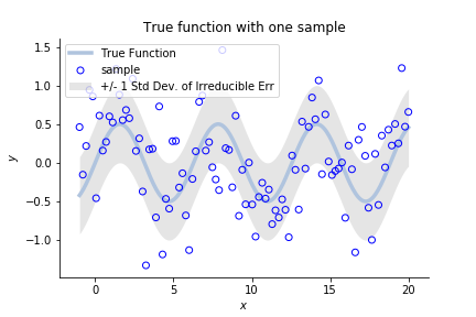 the true function \(f(x)\) to be estimated, along with the noise variance and sample observations
The dots represent a sampled dataset, like a column of \(\mathbf{Y}\). To repeat, we are to use it to infer \(f(x)\).
To do this, we’ll use a smoothed version of the \(k\)-nearest neighbor algorithm. In line with the above, we’ll do it on many samples and overlay each prediction curve over the true function. Then we’ll pick a particular \(x\)-value, labeled \(x_1\), and inspect the histogram of predictions for that point. This will reveal bias and variance.
Further, we’ll do this for multiple choices of the regularizing hyperparameter. In this case, it is something akin to the numbers of neighbors.
This can all be displayed with:
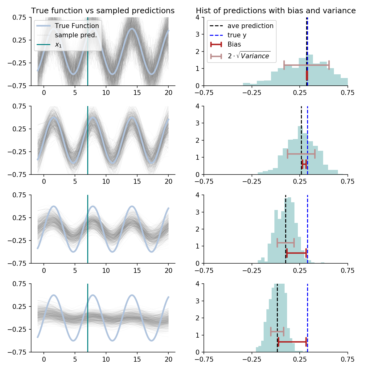 Left: Blue line is the true function. The small grey lines are prediction curves for different samples of data. Lower plots show prediction curves under stronger regularization. The green vertical line indicates the evaluation point, corresponding to the histograms on the right. \(\\\) Right: Histogram of predictions at \(x_1\) across data samples. The width of the distribution, a driver of overall error, is measured with variance. The difference between the histogram’s average and the true function is measured by bias.
Inspecting this, we see an estimating procedure optimized for bias is quick to accept the wave pattern, but is frequently mislead by noise. An estimating procedure optimized for variance hesitates to accept the waves, protecting itself from noise, but underestimating their amplitude. Somewhere in the middle is an estimating procedure that will perform best out of sample.
Finally, we end with two notes:
- The bias-variance decomposition is more useful than the assumptions suggest. It generalizes to different losses and even classification problems. It’s safe to say that for any modeling task, the bias-variance decomposition is relevant at some level. See P. Domingo (2000) for ideas on generalization the trade-off.
- In practice, we only observe a single column from \(\mathbf{Y}\). How can we optimize across columns in practice? The approach is to approximate what occurs across columns with what varies within the observed dataset. This is precisely what cross validation does.
If you’d like to learn more, see my video on this topic.
Appendix: Algebra for the Bias-Variance Decomposition
The bias-variance decomposition can be determined as follows:
\[\begin{align} \textrm{ExpErr}(\mathbf{x}_1) = & \,\mathbb{E}\big[\big(y_1-f_{\textrm{est}}(\mathbf{x}_1)\big)^2\big] \\ = & \,\mathbb{E}\big[\big((f(\mathbf{x}_1)+\epsilon_1)-f_{\textrm{est}}(\mathbf{x}_1)\big)^2\big] \\ = & \,\mathbb{E}\big[(f(\mathbf{x}_1)+\epsilon_1)^2\big] - 2\mathbb{E}[f_{\textrm{est}}(\mathbf{x}_1)(f(\mathbf{x}_1)+\epsilon_1)] + \mathbb{E}\big[f_{\textrm{est}}(\mathbf{x}_1)^2\big]\\ = & \,\sigma_\epsilon^2+f(\mathbf{x}_1)^2 - 2f(\mathbf{x}_1)\mathbb{E}[f_{\textrm{est}}(\mathbf{x}_1)] + \mathbb{E}[f_{\textrm{est}}(\mathbf{x}_1)^2] \\ & +\underbrace{\mathbb{E}[f_{\textrm{est}}(\mathbf{x}_1)]^2-\mathbb{E}[f_{\textrm{est}}(\mathbf{x}_1)]^2}_\text{Equals 0, so we may add it in.}\\ = & \,\sigma^2_\epsilon+ \big(\mathbb{E}[f_{\textrm{est}}(\mathbf{x}_1)]-f(\mathbf{x}_1)\big)^2 + \mathbb{E}\big[\big(f_{\textrm{est}}(\mathbf{x}_1)-\mathbb{E}[f_{\textrm{est}}(\mathbf{x}_1)]\big)^2\big] \end{align}\]References
-
T. Hastie, R. Tibshirani and J. H. Friedman. The Elements of Statistical Learning: Data Mining, Inference, and Prediction 2nd ed. New York: Springer. 2009.
-
P. Domingos. A Unified Bias-Variance Decomposition and its Applications. ICML. 2000
-
S. Fortmann-Roe. Understanding the Bias-Variance Tradeoff. 2012
Something to Add?
If you see an error, egregious omission, something confusing or something worth adding, please email dj@truetheta.io with your suggestion. If it’s substantive, you’ll be credited. Thank you in advance!
Footnotes
-
We consider the single point \(\mathbf{x}_1\) only because it simplifies the presentation. In actuality, a model would be evaluated with an average over many point. ↩