Part 3: Variational Inference
Posted: Updated:
In Part 2, we defined:
Inference: The task of answering queries of a fitted PGM.
Variational Inference (‘VI’) produces approximate answers, a necessary concession when the exact alternative is hopeless. It casts inference as an optimization problem, providing an efficient means, a new perspective and fortuitously, a useful quantity.
Before proceeding, it may help to review the Notation Guide, the Part 1 summary and optionally, the Part 2 summary.
The Problem with Exact Inference
The problem is that the Gibbs Table, a theoretical table that provides the unnormalized probabilities of all variable assignments according to a PGM, is too large to store. Even if it could be stored, its computations would take too long. Exact inference algorithms provide techniques to lessen the burden, but often not far enough. Approximate algorithms sacrifice exactness for large gains in tractability.
The Idea of Variational Inference
The idea is to select from a space of tractable distributions one that closely approximates \(P_M\). With one selected, we can perform inference on it rather than on \(P_M\). The tractability constraint ensures inference is feasible.
To do this, we need to determine the space, have a method to search it and have a metric that tells us how well one distribution approximates another. More specifically, suppose \(\mathcal{Q}\) is a space of distributions and let \(\textrm{Q}\) refer to any distribution from \(\mathcal{Q}\). We want:
\[\hat{\textrm{Q}} = \textrm{argmin}_{\textrm{Q} \in \mathcal{Q}} D(\textrm{Q},P_M)\]where \(D(\textrm{Q},P_M)\) is some yet-to-be-defined metric that tells us how dissimilar \(\textrm{Q}\) and \(P_M\) are. If \(D(\textrm{Q},P_M)\) is low, this implies \(\textrm{Q}\) and \(P_M\) are similar. With this, we can perform inference on \(\hat{\textrm{Q}}\) in place of \(P_M\).
Naturally we ask, how is dissimilarity of two distributions measured?
Kullback–Leibler Divergence
We should note the task’s strangeness. \(\textrm{Q}\) and \(P_M\) are distributions which map assignments to probabilities. They are not typical objects for which typical dissimilarity metrics apply.
The key comes from information theory with the concept of Kullback–Leibler (‘KL’) divergence . As desired, it receives two probability distributions and produces a nonnegative number, where a large value indicates large dissimilarity and a zero value indicates identical distributions. It is defined as:
\[\begin{align} \mathbb{KL}(\textrm{Q} \vert \vert P_M) = \sum_{\mathbf{x} \in \textrm{Val}(\mathbf{X})} \textrm{Q}(\mathbf{x}) \log \frac{\textrm{Q}(\mathbf{x})}{P_M(\mathbf{x})}\\ \end{align}\]Unlikely other familiar measures of dissimilar, the KL divergence is not symmetric. In general:
\[\mathbb{KL}(\textrm{Q} \vert \vert P_M) \neq \mathbb{KL}(P_M \vert \vert \textrm{Q})\]The question of which to use is resolved by \(P_M\)’s unweildiness; it makes \(\mathbb{KL}(\textrm{Q} \vert \vert P_M)\) considerably easier to work with.
The Components of KL divergence
If we re-express \(P_M(\mathbf{x})\) as \(\frac{1}{Z}\widetilde{P}_M(\mathbf{x})\), rearrange and label, we get:
\[\small \begin{align} \mathbb{KL}(\textrm{Q} \vert \vert P_M) & = \underbrace{\big(-\sum_{\mathbf{x} \in \textrm{Val}(\mathbf{X})} \textrm{Q}(\mathbf{x}) \log \widetilde{P}_M(\mathbf{x})\big)}_{\textrm{cross entropy}} - \underbrace{\big(-\sum_{\mathbf{x} \in \textrm{Val}(\mathbf{X})} \textrm{Q}(\mathbf{x}) \log \textrm{Q}(\mathbf{x})\big)}_{\textrm{entropy of Q}} +\log Z \\ & = \mathbb{H}[\textrm{Q},\widetilde{P}_M] - \mathbb{H}[\textrm{Q}] +\log Z \end{align}\]This higlights the components of KL divergence:
- Cross entropy , \(\mathbb{H}[\textrm{Q},\widetilde{P}_M]\), is a measure of dissimilarity. If it’s high, \(\textrm{Q}\) puts high probability on \(\mathbf{x}\)’s that \(\widetilde{P}_M\) suggests are rare1. If it’s low, they distribute their probability mass similarly.
- \(\textrm{Q}\)’s Entropy, \(\mathbb{H}[\textrm{Q}]\), measures uncertainty. High entropy implies \(\textrm{Q}\) has its probability spread out evenly. Low entropy implies it has concentrated probabilities on a small number of \(\mathbf{x}\)’s. See this post for an explanation of this metric.
- \(P_M\)’s log normalizer, \(\log Z\), cannot be impacted by the choice of \(\textrm{Q}\), and so we may ignore it.
Intuitively, to minimize \(\mathbb{KL}(\textrm{Q} \vert \vert P_M)\) is to find a \(\textrm{Q}\) that distributes its probability mass as similarly as possible to \(P_M\) and is otherwise maximally uncertain. The uncertainty component is to be conservative; if two distributions have the same cross entropy with \(P_M\), the KL divergence will favor that which is more uncertain and is accordingly less opinionated without reason.
Benefits of KL divergence
There are two notable benefits of using the KL divergence.
First, there’s no need to compute \(P_M(\mathbf{x})\), which would involve computing \(Z\), a summation over exponentially many terms and often in practice, a nonstarter. Rather, it suffices to work with \(\widetilde{P}_M(\mathbf{x})\); what we do will be as though we used \(P_M(\mathbf{x})\).
The second benefit also relates to \(Z\). Suppose we manage a perfect optimization and found a \(\hat{\textrm{Q}}\) with a KL divergence of zero2. This implies:
\[\mathbb{H}[\hat{\textrm{Q}}] - \mathbb{H}[\hat{\textrm{Q}},\widetilde{P}_M] = \log Z\]Since we presumably obtained \(\hat{\textrm{Q}}\) by optimizing the terms of the left side, we know their values and by this equation, we know \(Z\).
In reality, we won’t find a \(\hat{\textrm{Q}}\) with a KL divergence of zero. But the better we optimize, the closer this quantity will approach \(\log Z\):
\[\begin{align} \mathbb{H}[\textrm{Q}] - \mathbb{H}[\textrm{Q},\widetilde{P}_M] & \rightarrow \log Z \\ \textrm{ as }\mathbb{KL}(\textrm{Q} \vert \vert P_M) & \rightarrow 0 \end{align}\]In fact, it’s a lower bound. For all \(\textrm{Q}\), we have:
\[\mathbb{H}[\textrm{Q}] - \mathbb{H}[\textrm{Q},\widetilde{P}_M] \leq \log Z\]This is fortuitous:
Optimizing the KL divergence yields an approximation to \(Z\). Computing \(Z\) is a notorious challenge in machine learning. Knowing it, evening approximately, brings benefits beyond inference, such as a means of model selection .
The Mean Field Method
Two questions remain to be answered:
- What is the tractability space \(\mathcal{Q}\) of distributions to be searched?
- How is it searched?
Resolving these specifies a VI algorithm. Here, we will produce the Mean Field method.
First, what is \(\mathcal{Q}\)? A reasonable proposal is all distributions that can be expressed as products of univariate distributions, distributions of a single valriable. If there are \(w\) variables in \(\mathbf{X}\), we may express this as:
\[\{ \textrm{Q} \in \mathcal{Q} \textrm{ if Q}=\prod_{i=1}^w q_i(X_i)\textrm{ for some univariate }q_i(\cdot)'s\}\]Second, how is the space searched? Conveniently, the choice of \(D(\cdot,\cdot)\) and \(\mathcal{Q}\) are designed to make this easy. Since a \(\textrm{Q}\) is defined by a set of \(q_i\)’s and we are using KL divergence, the task is to find:
\[\textrm{argmin}_{\{q_i\}'s} \mathbb{KL}\big[\prod_i q_i\big \vert \big \vert P_M\big]\]To do this, we’ll use an algorithm that updates each \(q_i\) iteratively. This follows from the Gibbs Rule for \(P_M\) and minimizing the KL divergence with respect to one \(q_j\) while treating the others as fixed. That is, we update \(q_j\) by setting it to:
\[\begin{align} q_j(X_j) & = \frac{1}{Z_j}\exp\big(\sum_{i:X_j \in \mathbf{D}_i} \mathbb{E}_{\mathbf{D}_i - \{X_j\} \sim \textrm{Q}}\big[\log \phi_i(\mathbf{D}_i)\big]\big) \\ & = \frac{1}{Z_j}\exp\big(\sum_{i:X_j \in \mathbf{D}_i} \sum_{\mathbf{D}_i}\log \phi_i(\mathbf{D}_i)\big[\prod_{X_k \in \mathbf{D}_i - \{X_j\}} q_k(X_k)\big] \big) \\ \end{align}\]The derivation of these updates is a bit complicated3, but we can note:
- It’s remarkable that this update reduces KL divergence to the whole of \(P_M\), but we need only consider factors for which \(X_j\) is involved. This is what ‘\(i:X_j \in \mathbf{D}_i\)’ specifies. We owe the tractability of this approach to this fact.
- Since \(X_j\) is a single variable, it’s tractable to compute \(Z_j\).
After iteratively applying the updates until the approximation stops improving, we’ll have a set of distributions, \(\{\hat{q_i}\}_{i=1}^w\), that define the approximation \(\hat{\textrm{Q}}\) to \(P_M\). Further, this factored form makes for efficient inference.
An Example
Suppose the ‘intractable’4 \(P_M\) is a multivariate normal with two random variables (\(X_1\) and \(X_2\)) and some positive correlation5:
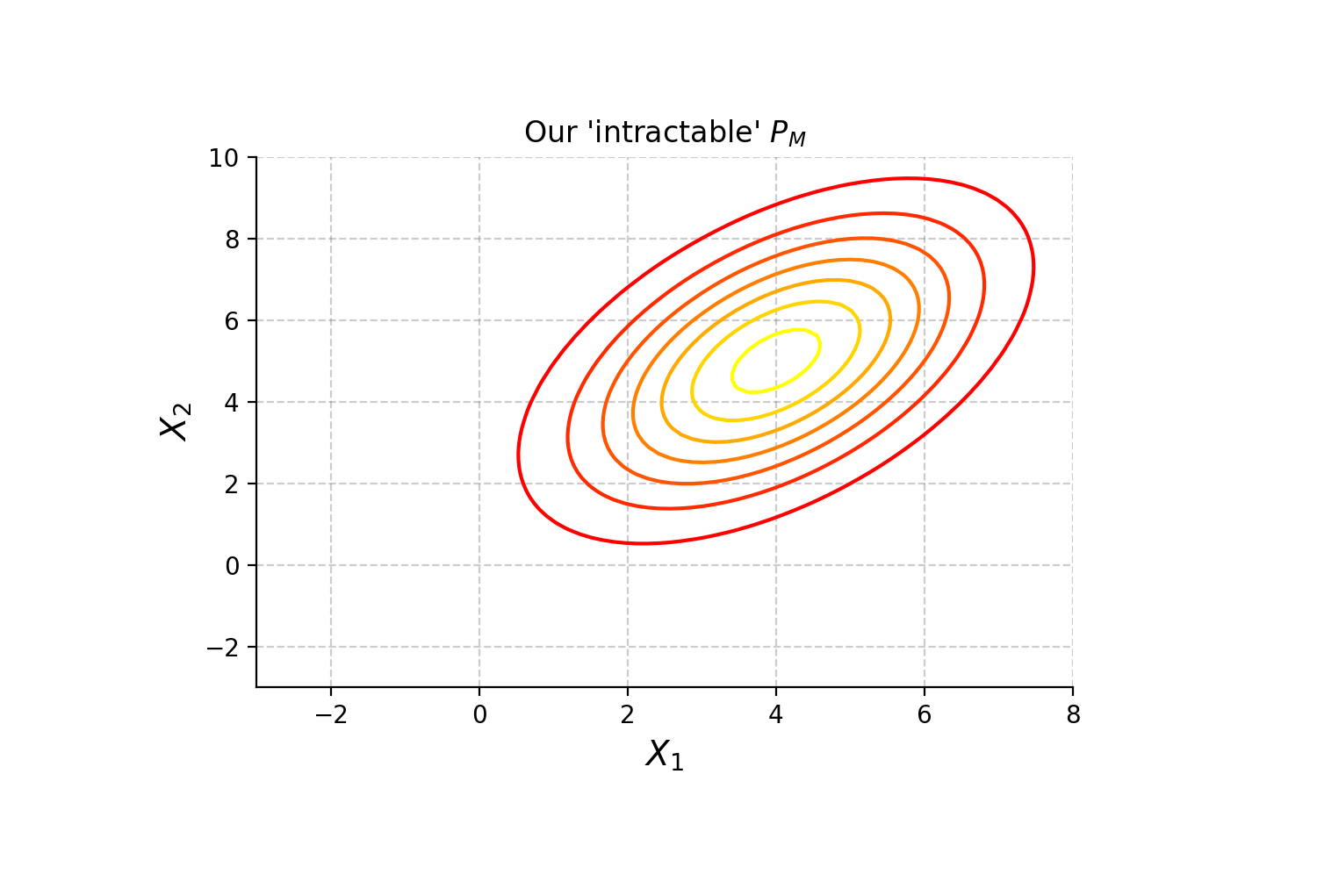
Next, suppose we initialize \(q_1(X_1)\) and \(q_2(X_2)\) as standard normal distributions. We overlay their product, the \(\textrm{Q}\) distribution, onto this graph and run the algorithm:
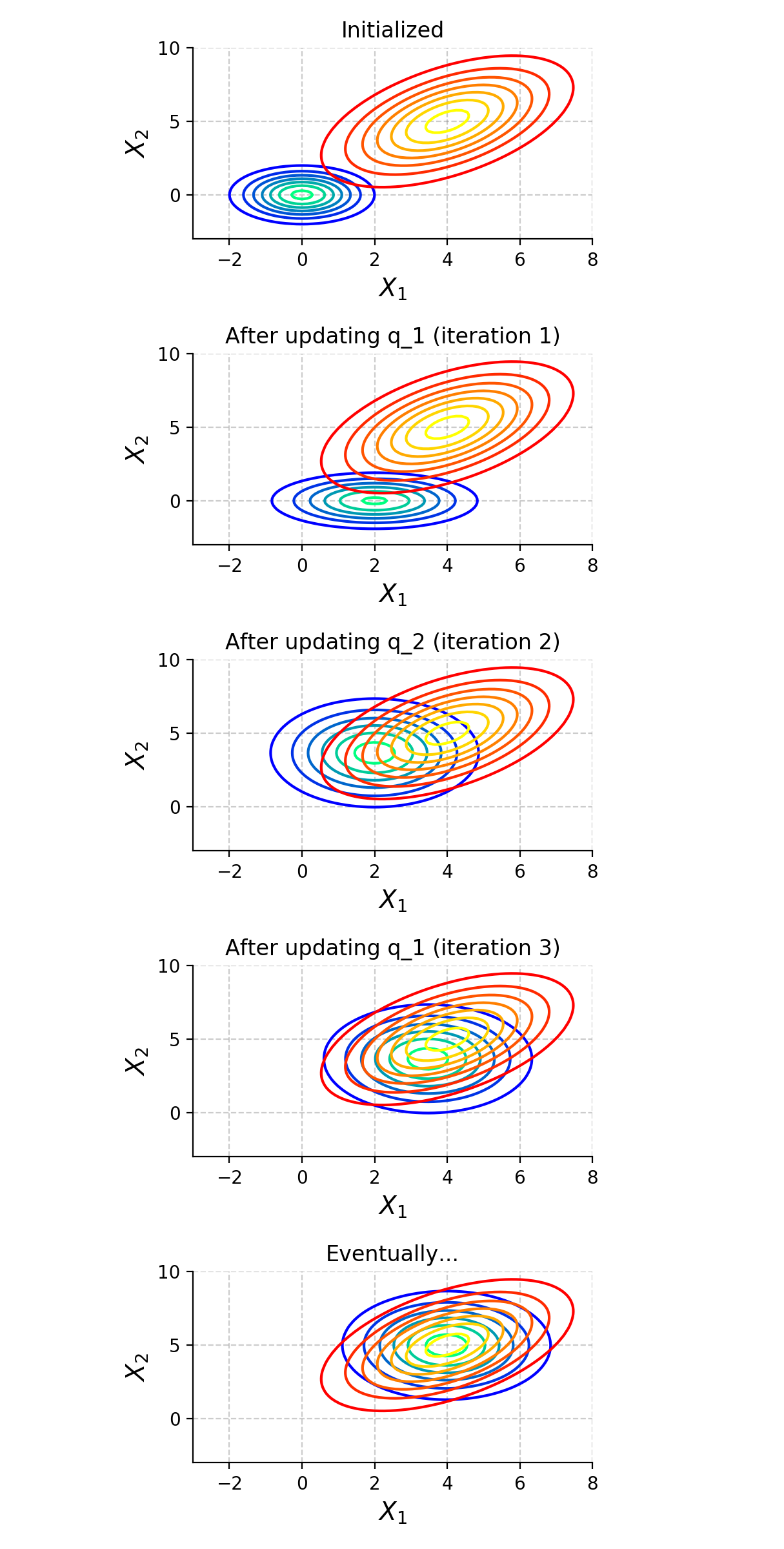 The Method Field method iteratively updates univariate factor distributions to approximate the target distribution.
As can be seen, the algorithm converges to the best choice of \(q_1\) and \(q_2\) for approximating \(P_M\).
Notice each update only impacts \(\textrm{Q}\) along one axis. This makes it a coordinate-descent-like algorithm, which can be slow to move in diagonal directions.
Further, notice the approximation doesn’t allow for joint behavior; the approximation fails to capture the correlation represented as \(P_M\)’s diagonal shape. This comes from the choice to use a product of univariate distributions, implying only independent behavior can be modeled. This is a major weakness of the Mean Field method.
The Broader View
We should be careful when generalizing the weaknesses of the Mean Field algorithm to the broader VI landscape. Will all VI algorithms be unable to express joint behavior? No, that fell out from our choice of \(\mathcal{Q}\). However, each will suffer whatever inexpressibility is created by the choice of tractable space. Will all VI algorithms slowly jitter to the target distribution if it’s in a diagonal direction? No, but a search bounded by some behavior is always necessary.
When considering VI, we should recall the three questions:
- How is the dissimilarity of distributions measured?
- What is the constrained space of tractable distributions?
- How is the space searched?
Answering these produces a specific VI algorithm, forces design trade-offs and makes alternative, candidate approaches clear.
The Next Step
If one is interested, there is an entirely different approach to approximate inference:
Otherwise, the next question concerns how the parameters are learned:
References
-
D. Koller and N. Friedman. Probabilistic Graphical Models: Principles and Techniques. MIT Press. 2009.
-
K. Murphy. Machine Learning: A Probabilistic Perspective. MIT Press. 2012.
-
M. Wainwright and M. I. Jordan. Graphical Models, Exponential Families, and Variational Inference. Foundations and Trends in Machine Learning. 2008.
Something to Add?
If you see an error, egregious omission, something confusing or something worth adding, please email dj@truetheta.io with your suggestion. If it’s substantive, you’ll be credited. Thank you in advance!
Footnotes
-
Technically, it’s not a valid cross entropy, since that applies to normalized distributions. In this case, we’re using an unnormalized distribution. ↩
-
This would imply \(\textrm{Q}\) is \(P_M\) in fact. ↩
-
See section section 21.3 of Murphy (2012) for the derivation. ↩
-
This is obviously not intractable, but suppose it is for illustrative purposes. ↩
-
Earlier I mentioned that everything is discrete and here I am, showing something continuous. Showing discrete visuals is tricky, so imagine this is a fine-grained discrete distribution. ↩