A Brief Explanation and Application of Gaussian Processes
Posted: Updated:
In supervised learning, we seek a function \(f(\cdot)\) that maps approximately from a feature vector \(\mathbf{x}\) to a prediction \(y\). Often that mapping is fixed by a choice of parameters \(\boldsymbol{\theta}\), informed by observed pairs \(\mathcal{D} = \{(\mathbf{x}_i, y_i)\}_{i=1}^N\). If we’re proper Bayesians, we determine probable functions by forming a posterior distribution over \(\boldsymbol{\theta}\).
Now consider how general this approach is. To appreciate, try to think of an approach that is outside this framework. That is, how might you determine a function \(f(\cdot)\) without relating it to a \(\boldsymbol{\theta}\) and performing a search over \(\boldsymbol{\theta}\)’s?
Hard right?1
Gaussian Processes, briefly
Gaussian Processes (‘GPs’) do this in an especially beautiful fashion.
Instead of determining a distribution over parameters, Gaussian Processes determine a distribution over functions.
Our first reaction should be, how is this possible? A function relates infinite inputs to infinite outputs. If we don’t have finite parameter vectors, how else do we corral these infinities?
Ultimately, it’s the Gaussian distribution that collapses the intractable infinite into the tractable finite. Specifically, we use a mathematical object called a Gaussian Process2, which allows us to reference functions by an arbitrary and finite set of input-output pairs.
Formally, we specify a Gaussian Process by writing:
\[f(\mathbf{x}) = GP(m(\mathbf{x}), \kappa(\mathbf{x},\mathbf{x}'))\]where \(m(\mathbf{x})\) and \(\kappa(\mathbf{x},\mathbf{x}')\) are pre-specified functions, called the mean function and the kernel function.
For intuition, take it as granted that we can sample from it a large number of function, \(f_1, f_2,\cdots, f_M\). If we evaluate these functions on an input \(\mathbf{x}^*\), then the average function output is \(m(\mathbf{x}^*)\). Further, if we evaluate these functions on two inputs \(\mathbf{x}_1\) and \(\mathbf{x}_2\), the covariance of outputs is \(\kappa(\mathbf{x}_1, \mathbf{x}_2)\). Consider these the definitions of the mean and kernel functions.
Just like we can sample a random variable, we can sample functions from a Gaussian Process. For example, if we specified \(m(\mathbf{x}) = 0\) and \(\kappa(\mathbf{x},\mathbf{x}')\) as the Matern Kernel, sampled functions look like:
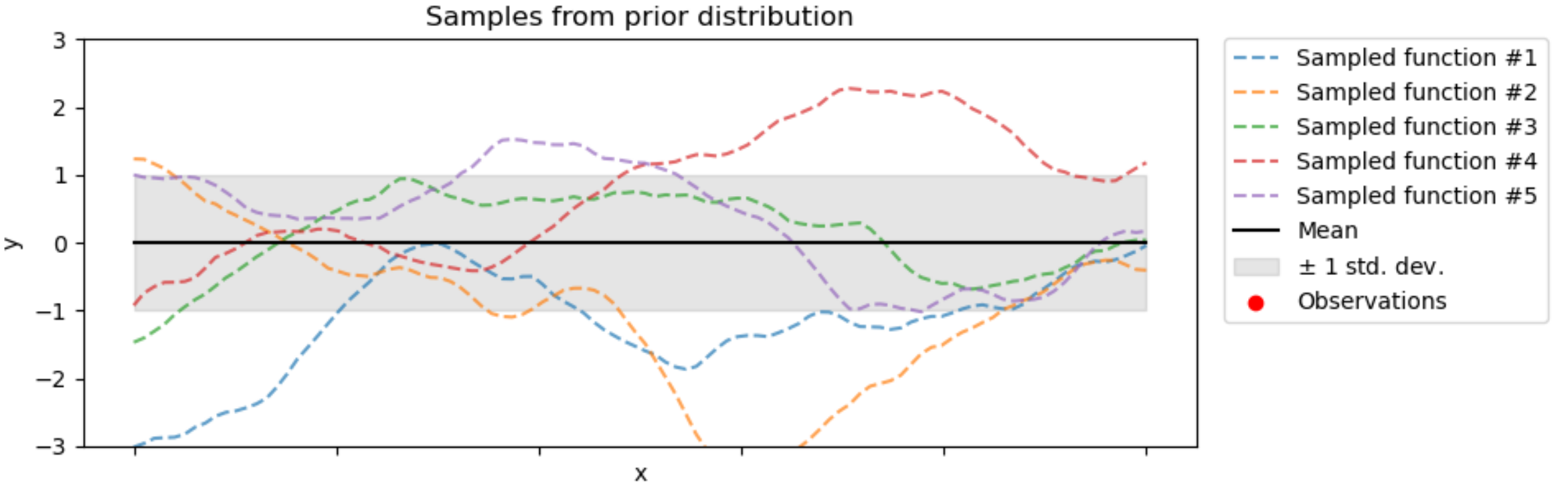
Credit: Scikit-Learn
With this idea, a GP model involves specifying a prior distribution over functions, which we’ll refer to as \(GP_{\textrm{prior}}\) . Then, using some Gaussian magic, we may condition on the data \(\mathcal{D}\) and determine a posterior distribution over functions, which we’ll refer to as \(GP_{\textrm{post}}\).
In implementation, we parameterize \(\kappa(\mathbf{x},\mathbf{x}')\)3 with a hyperparameter vector and choose one that maximizes agreement between the data and \(GP_{\textrm{prior}}\)4. The art in this technique comes down to selecting the appropriate kernel function. The guiding intuition is that a GP will produce similar outputs for kernel-similar inputs. It’s up to the artist to define kernel similarity consistent with the data.
In the end, we wield a fitted \(GP_{\textrm{post}}\), a rich probabilistic perspective on the data. Sampled functions are those in high agreement with the data. Functions that are unlikely per the data have a low probability of being sampled. Such posterior samples might look like:
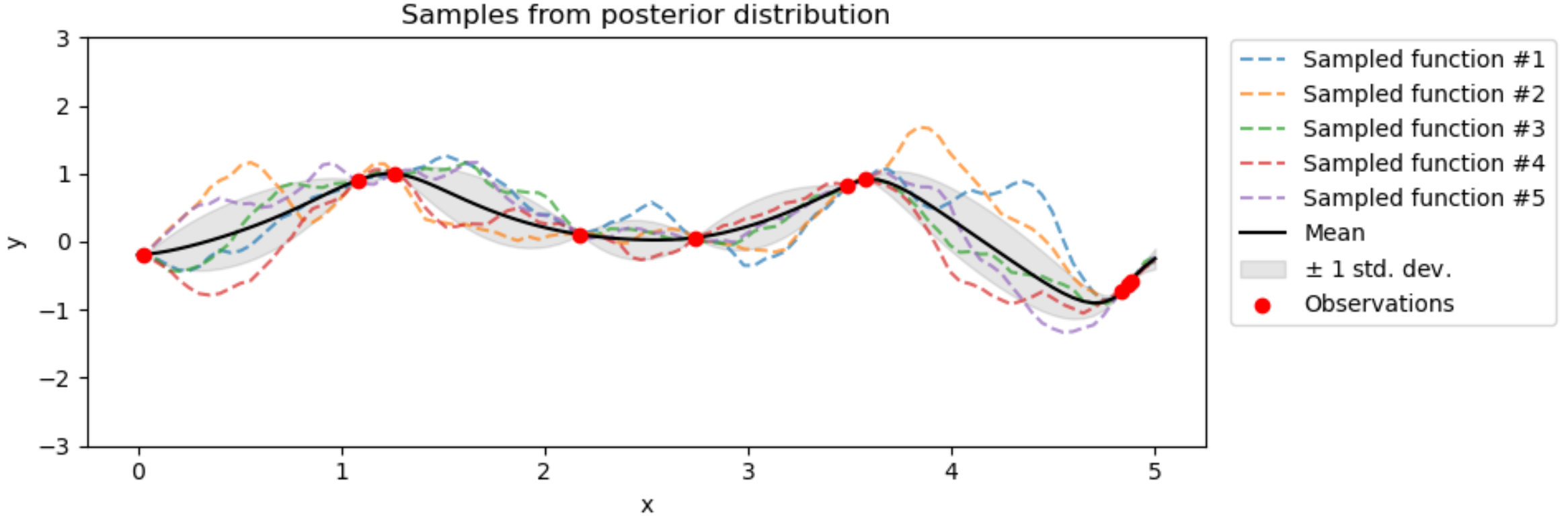
Credit: Scikit-Learn
Further, a prediction for a given \(\mathbf{x}^*\) is the average of all sampled functions evaluated at this point. This yields the black line above. Remarkably, it’s an integration over infinite outputs, enabled by Gaussian properties.
But averaging the outputs is an under utilization. These samples provide a distribution over outputs for any \(\mathbf{x}^*\). This can answer questions like:
- What is the probability the output of \(\mathbf{x}^*\) is within \([a, b]\)?
- What is the 90% credible interval of the output of \(\mathbf{x}^*\)?
An Application
To further our intuition, I’ll apply a GP to the prediction of my weight5 circa 2016, plotted below. I’ll focus on how to think about the problem and not about implementation. There is plenty of scikit-learn documentation for the latter.
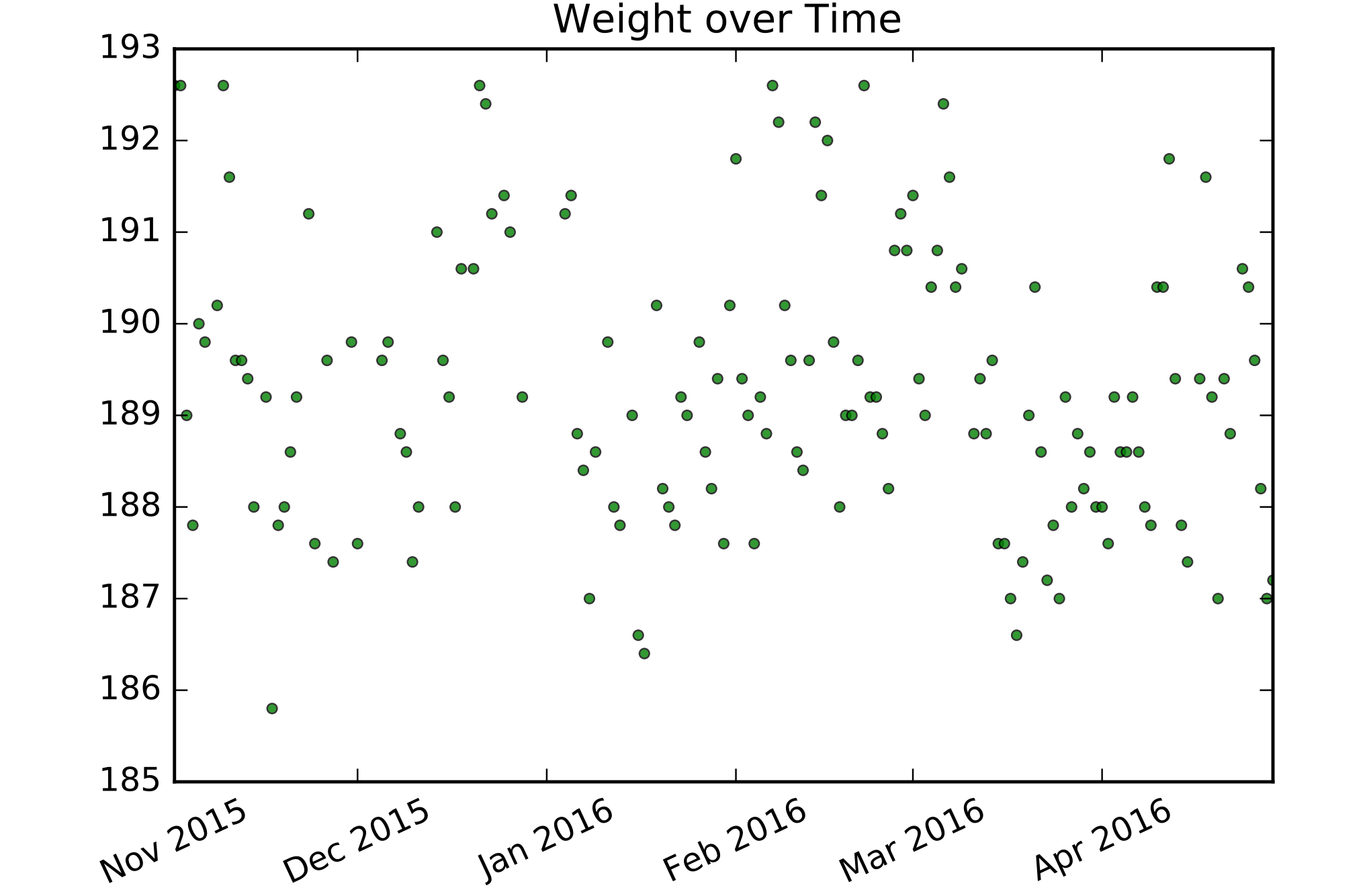
See a pattern? Me neither, but let’s ask: what about my ‘time’ feature dictates my weight? If I weigh myself twice, then those weights are likely to be similar if:
- Those moments in time are close.
- Those moments are in the same part of some cycle (same day of the week, year, etc.).
Fortunately, these are exactly the type of patterns that are easy to build into a kernel.
On top of that, the time feature likely isn’t the only factor. If we understand there are other influences outside the features, we shouldn’t expect to have full explanatory power. So we anticipate noise, which we may also build into the kernel.
Lastly, there is likely some longer term trending irregularity. Maybe I’m over supplied on spaghetti for two weeks. Maybe I got sick for a few days and lost a few pounds. Nothing in the time feature could predict this, but the distributions over functions should be flexible to fit it in sample. Flexibility in this regard relieves the fit-pressure on other effects (for example, the periodicity I mentioned) and prevents irregular trends from propagating out of sample. To do that, we use the Matern Kernel, as seen earlier.
With that, let’s test it using the latest 15% of the data. I’ll plot predictions along with one and two standard deviation confidence intervals. We get:
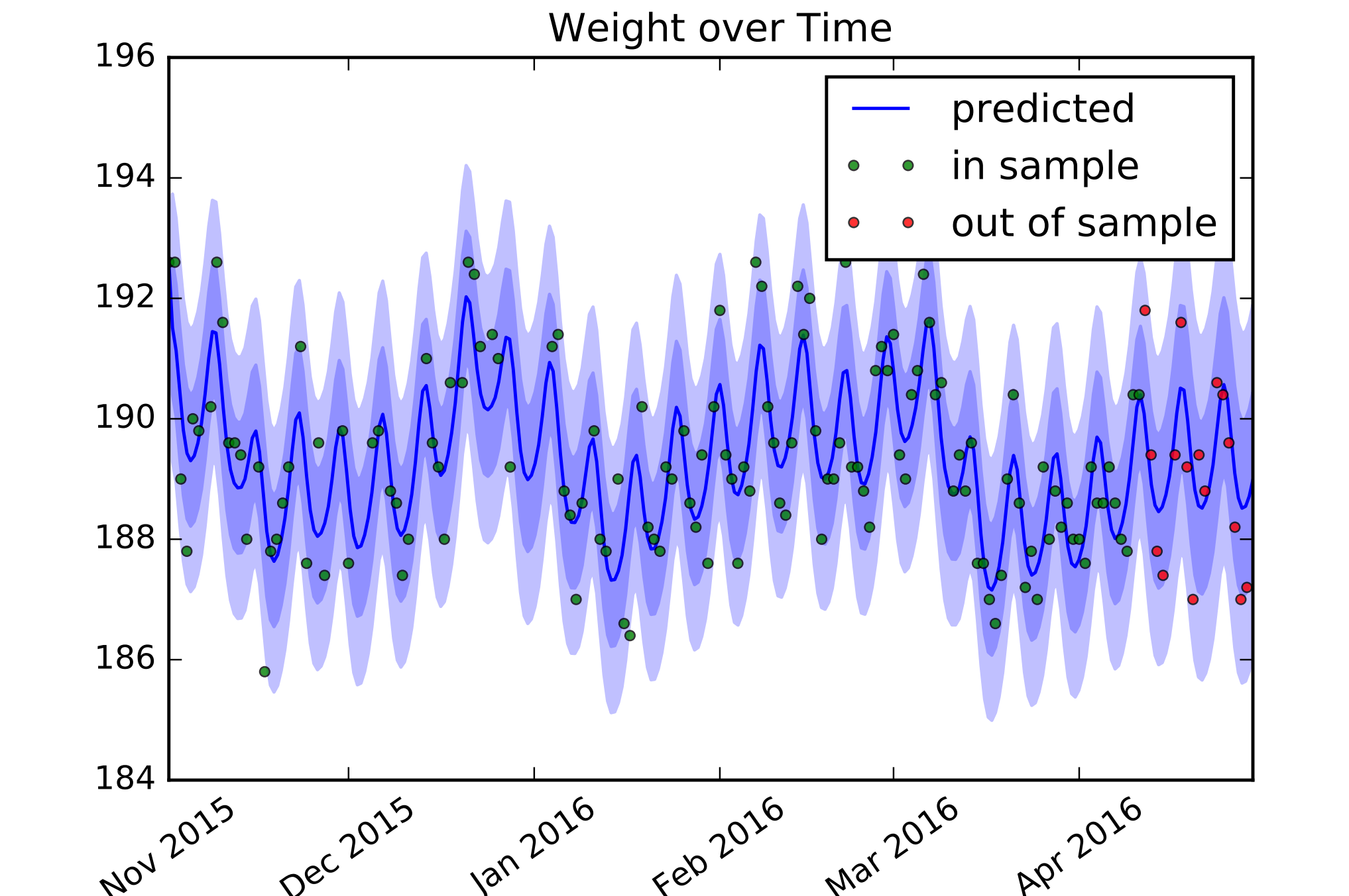
Now the pattern is clear. My weight has a roughly weekly periodicity and tends to trend over a few weeks, as is permitted by a Matern-induced function. Out of sample, we get decent predictions because it relies on the periodicity and doesn’t extrapolate out from spurious trending. The distributional output appears6 fairly well calibrated.
In summary
To conclude, Gaussian Processes are supremely clever, flexible and satisfying. They are certainly not universal tools, as they do not scale well7, but they are excellent for inserting intuitions into smaller problems.
And if you find this explanation disappointingly brief, I have a more expansive video on the topic.
References
-
C. E. Rasmussen and C. K. I. Williams. Gaussian Processes for Machine Learning. MIT Press. 2006.
-
D. Barber. Bayesian Reasoning and Machine Learning. Cambridge University Press. 2012.
-
D. Duvenaud. Automatic Model Construction with Gaussian Processes. University of Cambridge. 2014.
Something to Add?
If you see an error, egregious omission, something confusing or something worth adding, please email dj@truetheta.io with your suggestion. If it’s substantive, you’ll be credited. Thank you in advance!
Footnotes
-
Any non-parametric algorithm, where \(\boldsymbol{\theta}\) varies in size, counts as an answer. ↩
-
Confusingly, the ML technique and this mathematical object have the same name. ↩
-
Demeaning the \(y_i's\) is normally sufficient for setting \(m(\mathbf{x}) = 0\). The kernel function is flexible enough to capture all other input-output behavior. ↩
-
This amounts to model selection a la Empirical Bayes. ↩
-
I’m using my weight because I’m familiar with what explains it. ↩
-
We don’t have enough out of sample data to well validate the calibration, so I’m being generous here. ↩
-
The vanilla application of GPs incurs a \(O(N^3)\) cost, coming from the inversion of an \(N\)-by-\(N\) kernel similarity matrix. Much research has been invested to bring this cost down, but all with some sacrifice of approximation. ↩