The Exponential Family
Posted: Updated:
The1 exponential family generalizes a large space of distributions, and those included share the family’s remarkable properties. To see this, we’ll start in familiar territory, the Normal distribution. We’ll see how it’s created by setting the dials of the exponential family and how adjusting those dials sweeps over a wide and appealing universe of objects. We end with a discussion of one of its notable properties, providing one reason it’s a favorite modeling abstraction.
Familiar Territory
Let’s consider a list of numbers that look Normally distributed. The goal is to determine which distribution matches these numbers. That is, we speculate a distribution, the Normal in this case, and determine the parameters that make the most sense according to the data. ‘Make the most sense’ translates to picking the maximum likelihood estimate (‘MLE’).
Before one shouts ‘use the empirical mean and variance!’, let’s understand that suggestion’s purpose. At bottom, we seek parameters \(\mu\) and \(\sigma^2\) that maximize the likelihood of the data:
\[\mu^*,\sigma^{2*} = \textrm{argmax}_{\mu,\sigma^2} \prod_i^N \mathcal{N}(x_i \vert \mu,\sigma^2)\]It turns out the answer is easy to compute; it’s the empirical mean and variance. However, that solution doesn’t generalize2 simply, so we ignore it. Instead, let’s scan for values of \(\mu\) and \(\sigma^2\) until we find a combination that yields a distribution that best matches the histogram of numbers:
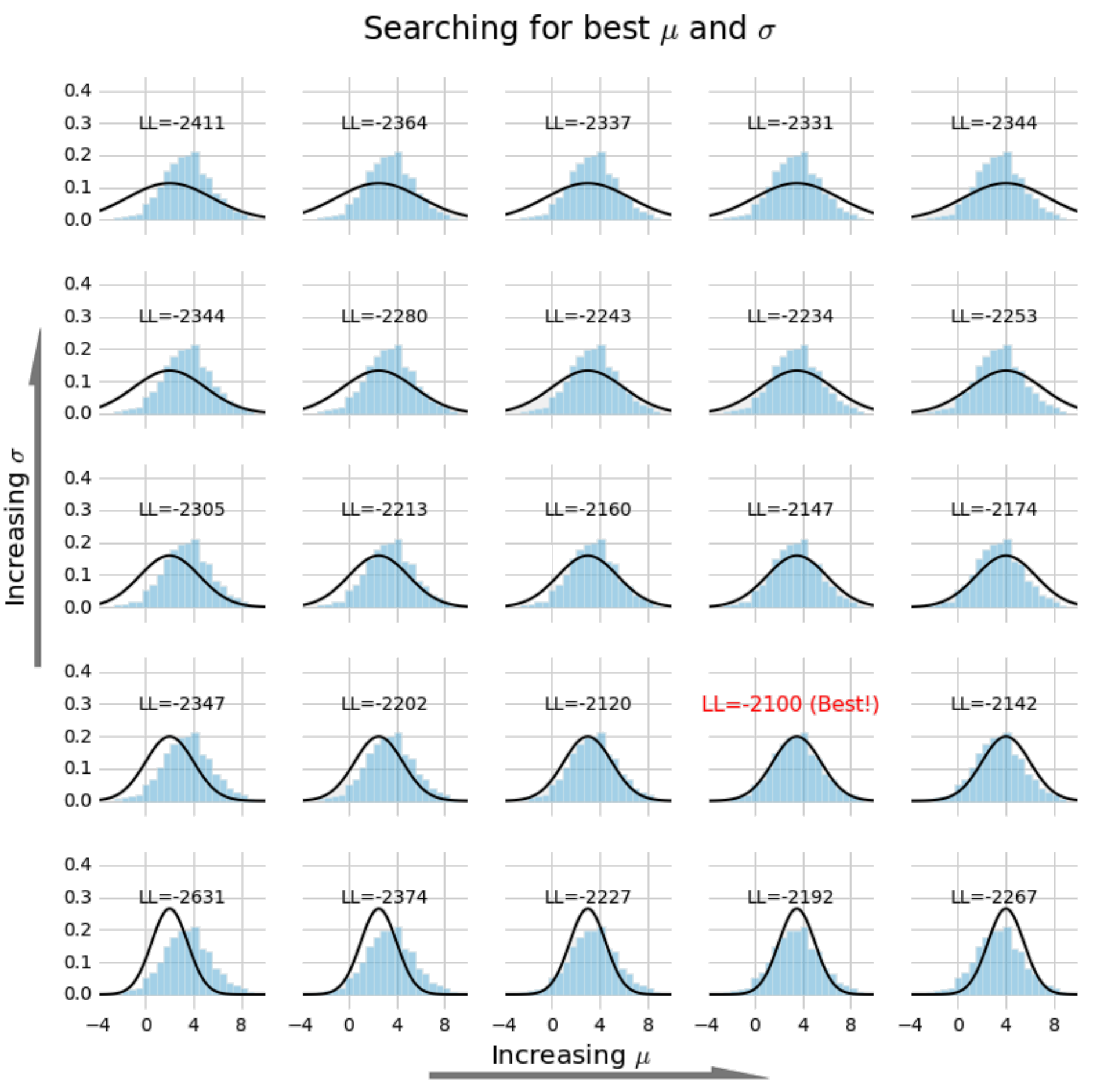 Different choices of parameters provide different fits to the data. Choosing those which maximize the log-likelihood (indicated with ‘LL’) provides a fit to the data.
Now we’ll do the exact same thing, but with a rewrite of the algebra:
\[\begin{align} \mathcal{N}(x_i \vert \mu,\sigma^2) = & \frac{1}{\sqrt{2\pi\sigma^2}}\exp\Big({-\frac{(x_i-\mu)^2}{2\sigma^2}}\Big) \\ = & \exp\Big(\frac{\mu}{\sigma^2}x_i - \frac{1}{2\sigma^2}x_i^2 - \frac{1}{2\sigma^2}\mu^2-\log\sigma -\frac{1}{2}\log (2\pi) \Big) \\ = & \exp\Big(\left[\begin{array}{cc} x_i & x_i^2\end{array}\right]\left[\begin{array}{c} \frac{\mu}{\sigma^2}\\ -\frac{1}{2\sigma^2} \end{array}\right] - \big(\frac{1}{2\sigma^2}\mu^2+\log\sigma + \frac{1}{2}\log (2\pi) \big)\Big) \\ \end{align}\]We relabel:
\[\left[\begin{array}{c} \frac{\mu}{\sigma^2}\\ -\frac{1}{2\sigma^2} \end{array}\right] = \left[\begin{array}{c} \theta_1\\ \theta_2 \end{array}\right]\]It’s clear that if we know \(\theta_1\) and \(\theta_2\), we also know \(\mu\) and \(\sigma^2\). So we may reason in these terms; instead of searching for \(\mu\) and \(\sigma^2\), we seek \(\theta_1\) and \(\theta_2\):
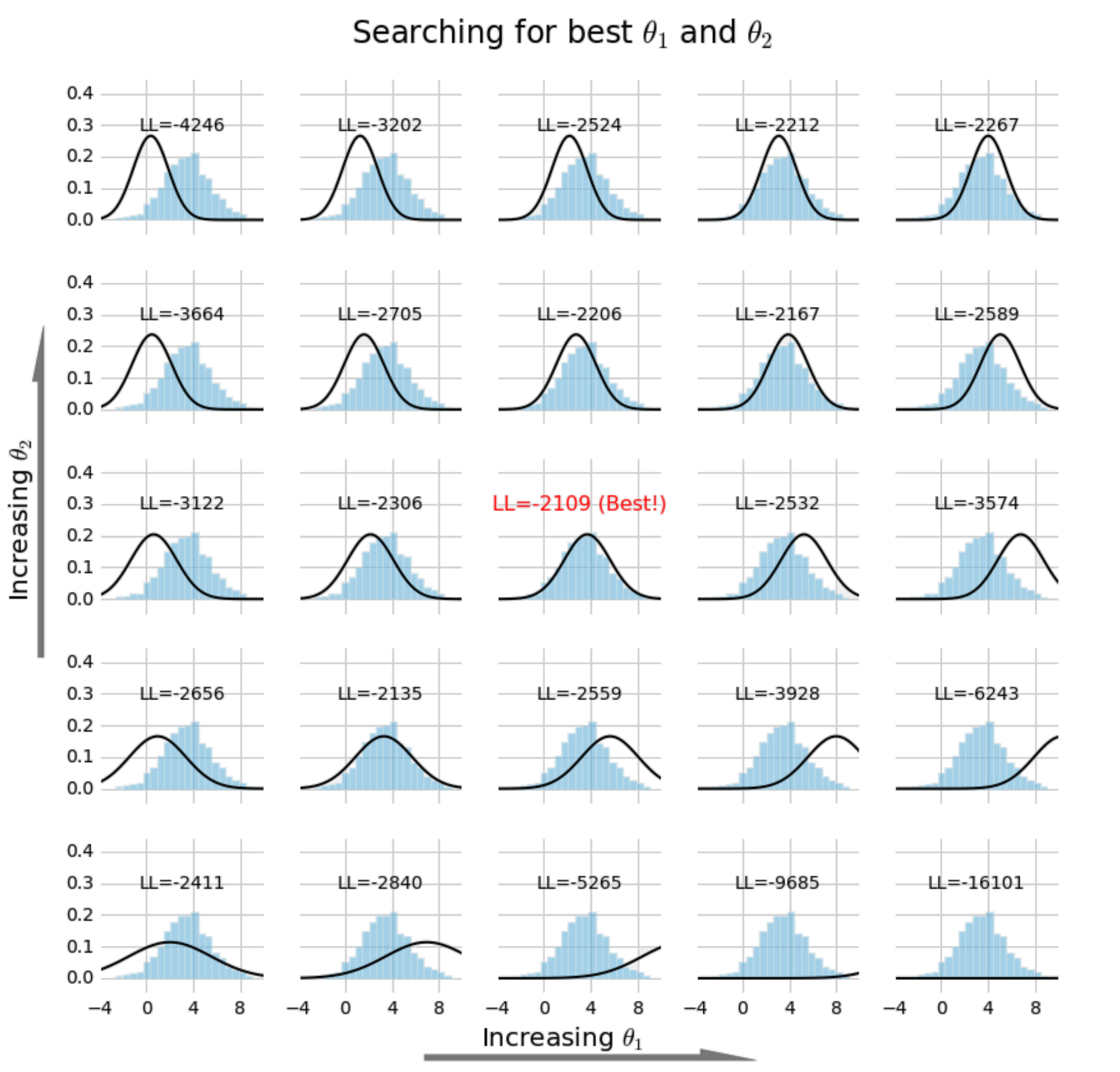 This is the same search as performed above, except it’s in terms of \(\theta_1\) and \(\theta_2\).
A natural question is: Why did we do this? It’s because a huge space of distributions can be written in this form. We can do the equivalent of finding \(\mu^*\) and \(\sigma^{2*}\), but for a set far beyond the Normal.
Defining the Exponential Family and its Components
Now we define the exponential family. At first blush, it appears heavy and abstract, but we’ll come to see it merely presents several choices.
With a distribution from the exponential family, the probability mass or density of a vector \(\mathbf{x}\) according to a parameter vector \(\boldsymbol{\theta}\) is:
\[\begin{align} p(\mathbf{x} \vert \boldsymbol{\theta})=&\frac{1}{Z(\boldsymbol{\theta})}h(\mathbf{x})\exp\Big({T(\mathbf{x})\cdot\boldsymbol{\theta}\Big)}\\ \end{align}\]
\(Z(\boldsymbol{\theta})\) is called the partition function and ensures \(p(\mathbf{x}\vert\boldsymbol{\theta})\) sums to one over the domain of \(\mathbf{x}\). That is:
\[Z(\boldsymbol{\theta}) = \int h(\mathbf{x})\exp\Big({T(\mathbf{x})\cdot\boldsymbol{\theta}\Big)} \nu(d\mathbf{x})\]\(\nu(d\mathbf{x})\) refers to the measure of \(\mathbf{x}\). It generalizes the operation of ‘summing over all possible events’ to multiple domain types: discrete, continuous or subsets of either. To select \(\nu(d\mathbf{x})\) is to know how to sum over all possible \(\mathbf{x}\) values. It also may determine the ‘volume’ of \(\mathbf{x}\), though that could equivalently be captured with \(h(\mathbf{x})\).
In fact, let’s declare that separation; \(h(\mathbf{x})\) is the volume of \(\mathbf{x}\). One may think of it as the component of \(\mathbf{x}\)’s likelihood that is not due to the parameters. This will become clear with an example.
\(T(\mathbf{x})\) is called the vector of sufficient statistics. This is a measurement that includes everything the parameters care about when determining the likelihood of \(\mathbf{x}\). In other words, if two vectors have the same sufficient statistics, then all the other ways in which they may be different do not change their likelihood in the eyes of the parameters3.
We need to cover a few extra details regarding the parameters:
-
We consider only the space of parameters for which the partition function is finite. If we inspect \(Z(\boldsymbol{\theta})\), it’s easy to imagine an integral that diverges. This space of valid parameters is called the natural parameter space.
-
There should be no linear dependencies between the parameters (or sufficient statistics) in this representation, meaning we should be free to move all elements of \(\boldsymbol{\theta}\). Said differently, knowing one subset of parameters should never fix the others. If this is true, the representation is said to be minimal. There are a two reasons for this. First, we lose no capacity for representing distributions by enforcing it. Second, since we will ultimately be searching over the space of \(\boldsymbol{\theta}\), we will have the benefit that different \(\boldsymbol{\theta}\)’s always imply different distributions.
The second bullet will guide how we should think; the length of \(\boldsymbol{\theta}\) will determine how many degrees of freedom we have over the probability distributions. So when we determine \(T(\mathbf{x})\), we need to first think carefully about its length.
The Dataset’s Likelihood
At this point, we notice something useful. In this form, consider how the probability of a sample combines to form the probability of the entire dataset:
\[\begin{align} \prod_i^N p(\mathbf{x}_i \vert \boldsymbol{\theta}) & =\prod_i^N h(\mathbf{x}_i)\exp\Big({T(\mathbf{x}_i)\cdot\boldsymbol{\theta}-\log Z(\boldsymbol{\theta})\Big)} \\ & = \underbrace{\Bigg[\prod_i^N h(\mathbf{x}_i)\Bigg]}_{h_N(\mathbf{X})}\exp\Big({\underbrace{\big(\sum_i^N T(\mathbf{x}_i)\big)}_{T_N(\mathbf{X})}\cdot\boldsymbol{\theta}-N\log Z(\boldsymbol{\theta})\Big)} \\ \end{align}\]This labeling demonstrates that if each data point is modeled using the exponential family, then the entire dataset is also modeled from within the exponential family.
Since determining the MLE will involve maximizing the log of this, we define:
\[\mathcal{L}_N(\boldsymbol{\theta}) \stackrel{\text{def}}{=} \log \prod_i^N p(\mathbf{x}_i \vert \boldsymbol{\theta})\]The Normal Distribution as a Special Case
When we fit the Normal distribution, we were silently making choices with respect to the exponential family. Those were:
- \(x\) could be any real number. This fixes \(\nu(dx)\) and thus determines how we’ll do the integration; we’ll integrate over the real line.
- \(x\) is Normally distributed, which dictates a few things:
- It has two degrees of freedom, which is the length of \(T(x)\) and \(\boldsymbol{\theta}\).
- \(T(x) = [x,x^2]\), which means probabilities are influenced by parameters only via a linear relationship with these measurements.
- \(h(x) = 1\), which means the difference in likelihood between two \(x\) values is due entirely to the parameters. In other words, all \(x\)’s are of the same size.
From here, the definition of the exponential family will dictate the rest:
\[\begin{align} Z(\boldsymbol{\theta}) = & \int h(\mathbf{x})\exp\Big({T(\mathbf{x})\cdot\boldsymbol{\theta}\Big)} \nu(d\mathbf{x})\\ = & \int \exp\Big({ \left[\begin{array}{cc} x & x^2\end{array}\right] \cdot \left[\begin{array}{c} \theta_1\\ \theta_2 \end{array}\right] \Big)} dx \\ = & \exp\Big( \frac{-\theta^2_1}{4\theta_2} - \frac{1}{2}\log(-2\theta_2) - \frac{1}{2}\log(2\pi)\Big) \end{align}\]Since we’re interested in the MLE parameters, we can determine \(\mathcal{L}_N(\boldsymbol{\theta})\):
\[\begin{align} \mathcal{L}_N(\boldsymbol{\theta}) = & \sum_i^N\log \mathcal{N}(x_i \vert \mu,\sigma^2) \\ = & \left[\begin{array}{cc} \sum_i^N x_i & \sum_i^N x_i^2\end{array}\right]\left[\begin{array}{c} \theta_1\\ \theta_2 \end{array}\right] - N\big( \frac{-\theta^2_1}{4\theta_2} - \frac{1}{2}\log(-2\theta_2) - \frac{1}{2}\log(2\pi)\big) \end{align}\]From here, picking the best \(\theta_1\) and \(\theta_2\) (maximizing \(\mathcal{L}_N(\boldsymbol{\theta})\)) is the same procedure we did earlier.
In Full Generality
The definition shows its flexibility. We didn’t need to say \(x\) was real valued; that was our choice. We didn’t need to say the sufficient statistics were \([x,x^2]\), we could have picked anything. To demonstrate this range, let’s say we’re faced with data like this:
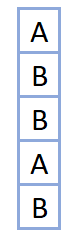 some categorical data
The challenge is the data’s non-numeric nature. To handle it, we can choose as follows:
- \(\nu(dx)\) should mean we sum over the two possible outcomes: \(x=A\) and \(x=B\).
-
Given the data’s low cardinality, one degree of freedom is appropriate. Under this constraint, the indicator function is a natural choice:
\[T(x)= \mathbb{I}[x=A] = \begin{cases} 1 & \text{if } x = A\\ 0 & \text{if } x = B \end{cases}\] - Outside of something that relates to the parameters, there is no reason to think \(x=A\) has a different intrinsic, probabilistic volume than \(x=B\), so we set \(h(x)=1\).
With these choices, what does that imply for \(Z(\boldsymbol{\theta})\)?
\[\begin{align} Z(\theta) = & \int h(x)\exp\Big({T(x)\cdot\theta\Big)} \nu(dx)\\ = & \int \exp\Big({\mathbb{1}[x=A]\cdot\theta\Big)} \nu(dx)\\ = & \sum_{x \in \{A,B\}} \exp\Big({\mathbb{1}[x=A]\cdot\theta\Big)}\\ = & \exp(\theta) + 1 \end{align}\]Next, we can write \(p(x\vert\theta)\):
\[\begin{align} p(x \vert \theta)= &\frac{1}{Z(\theta)}h(x)\exp\Big({T(x)\cdot\theta\Big)}\\ = &\frac{1}{\exp(\theta) + 1}\exp\Big({\mathbb{1}[x=A]\cdot\theta\Big)}\\ \end{align}\]Or, more explicitly:
\[\begin{align} p(x=A \vert \theta) = &\frac{\exp(\theta)}{\exp(\theta) + 1}\\ p(x=B \vert \theta) = &\frac{1}{\exp(\theta) + 1} = 1 - p(x=A \vert \theta) \end{align}\]Since we may choose \(\theta\) such that \(p(x=A\vert\theta)\) is any value in \((0,1)\), we realize we’ve arrive at the Bernoulli distribution.
To pick the most likely parameters, we optimize \(\mathcal{L}_N(\theta)\), just like we did in the case of the Normal. In this case, there is an analytic solution. \(\theta^*\) is such that \(p(x=A\vert\theta^*)\) matches the empirical proportion where \(x = A\).
We see, one set of choices led us to the Normal distribution while another led us to the Bernoulli.
Trickier Data
What if we came across data like this:
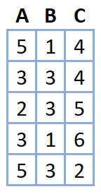 counts of categories
This appears trickier. \(\mathbf{x}\) is a length 3 vector with the unusual constraint of summing to 10. Again, the problem is solved with proper choices:
- What is \(\nu(d\mathbf{x})\)? How should we think about all possible events that we should sum over? Or, what are all possible observations we could come across? It’s any 3 nonnegative integers such that their sum is 10. Those are:
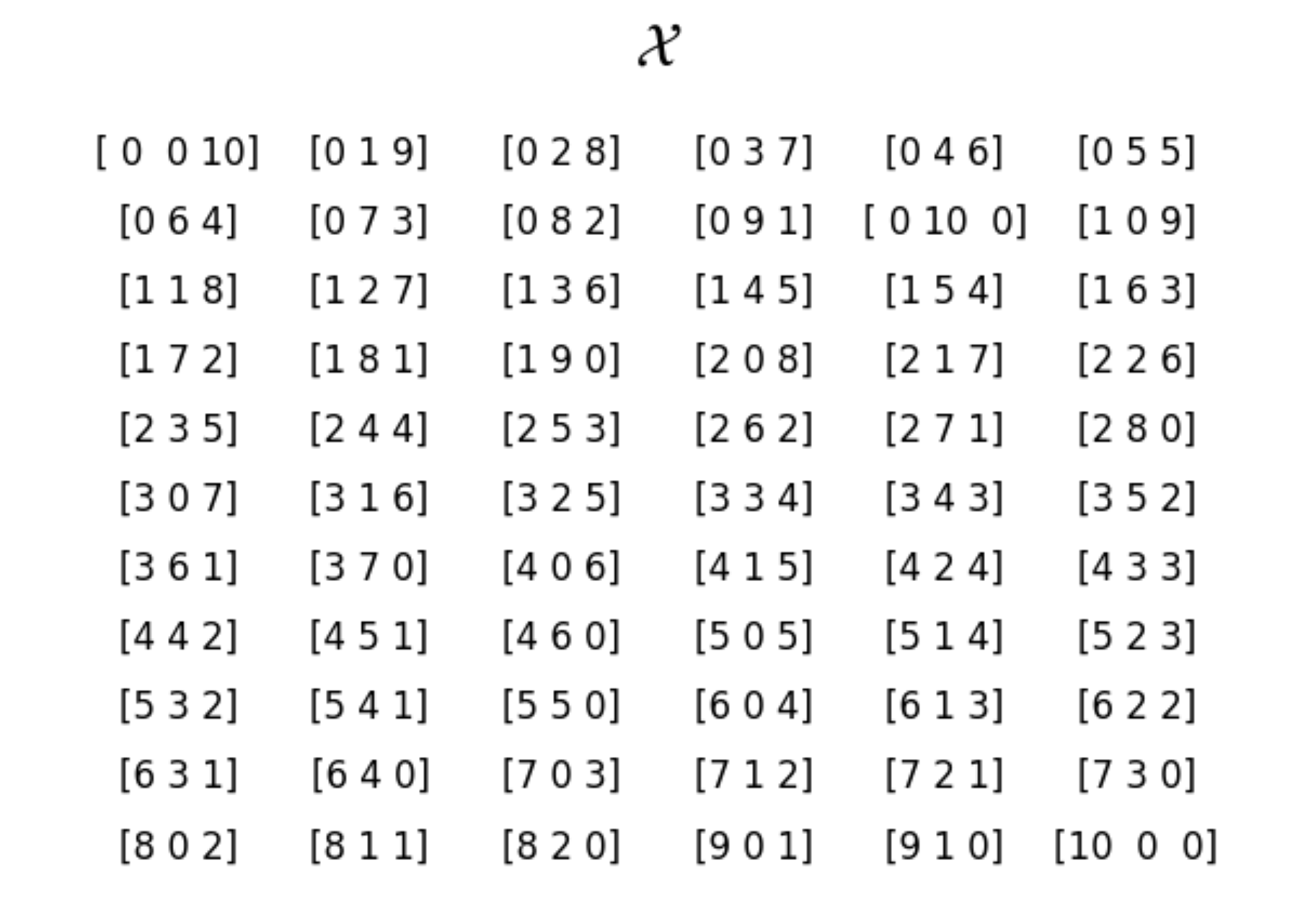 The set of all length 3 nonnegative integers that sum to 10.
This is the set to sum over. We’ll call it \(\mathcal{X}\).
-
How many degrees of freedom should the distribution allow? It’s reasonable to suspect a parameter for each column, but the sum-to-10 constraint will subtract one. Therefore, we’ll say there are two degrees of freedom.
-
What is \(T(\mathbf{x})\)? The most natural choice is the data itself. We may use the first two elements of \(\mathbf{x}\). We aren’t losing information regarding the last element, since the distribution will also ‘know’ that the sum is 10.
-
What is \(h(\mathbf{x})\)? In other words, should one observation of \(\mathbf{x}\) ever be considered more likely than another, regardless of the parameters?
To answer this, consider how we would generate an observation of \(\mathbf{x}\). One way is to make 10 draws from some distribution and aggregate the results. For example, \(AABBCABABC \implies [4,4,2]\). The utility is that all possible sequences map to all of \(\mathcal{X}\). From this angle, do some observations seem more likely than others, even though we can’t reference the distribution that generates a single draw? Yes, since some observations are mapped to by more sequences than others. For example, the only thing that maps to \([10,0,0]\) is \(AA \cdots A\) while \([9,1,0]\) is mapped to by 10 sequences (\(BA\cdots A\), \(AB\cdots A\), \(\cdots\), \(AA\cdots B\)). It appears the latter observation is 10 times bigger than the former. Notice this is true despite not knowing the parameters. That is, it’s true regardless of the categorical distribution from which we drew the sequence. Ultimately, this suggest we set \(h(\mathbf{x})\) to the number of sequences that map to \(\mathbf{x}\). Specifically:
With the choices set, we can determine the partition function:
\[\begin{align} Z(\boldsymbol{\theta}) = & \int h(\mathbf{x})\exp\Big({T(\mathbf{x})\cdot\boldsymbol{\theta}\Big)} \nu(d\mathbf{x})\\ = & \sum_{\mathbf{x}\in \mathcal{X}} \frac{10!}{x_1!x_2!x_3!}\exp\Big(\mathbf{x}_{:2}\cdot\boldsymbol{\theta}\Big)\\ = & (\exp(\theta_1) + \exp(\theta_2) + 1)^{10} \end{align}\]Next, we may write the expression for the probability:
\[\begin{align} p(\mathbf{x} \vert \boldsymbol{\theta}) = & \frac{1}{(\exp(\theta_1) + \exp(\theta_2) + 1)^{10}}\frac{10!}{x_1!x_2!x_3!}\exp\Big(\mathbf{x}_{:2}\cdot\boldsymbol{\theta}\Big)\\ \end{align}\]At this point, we have everything necessary to optimize \(\mathcal{L}_N(\boldsymbol{\theta})\).
However, we’ve seemingly not landed on a familiar distribution, as we had in previous cases. Indeed, this is an unusual expression. Fortunately, the appearance is merely a consequence of the derivation. It’s in fact equivalent to:
\[p(\mathbf{x} \vert \boldsymbol{\theta})= \frac{10!}{x_1!x_2!x_3!}p_1^{x_1}p_2^{x_2}p_3^{x_3}\]where \(\theta\) has been rewritten in terms of probabilities \(p_1\), \(p_2\) and \(p_3\). These are the probabilities of drawing each category in the sequence generating construction. Ultimately, this is the Multinomial distribution.
Beyond the Examples
To fully appreciate the range of the exponential family, we view the following table, displaying distributions produced by choices of \(h(\mathbf{x})\) and \(T(\mathbf{x})\):
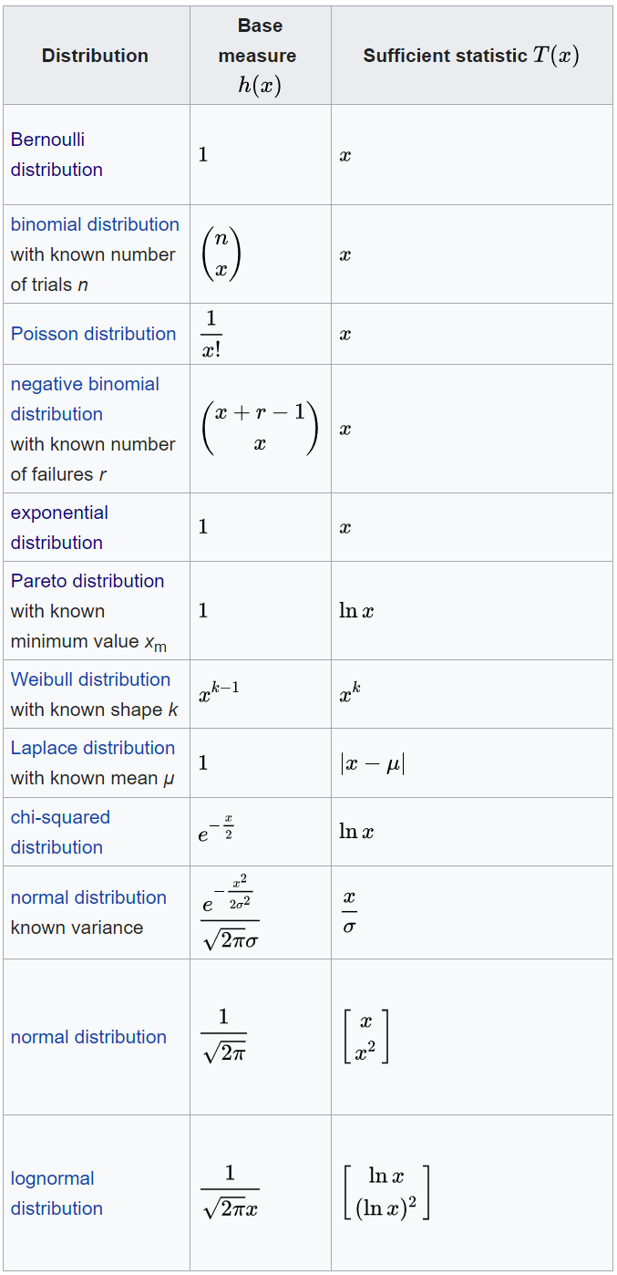 The distributions given by different choices of \(h(\mathbf{x})\) and \(T(\mathbf{x})\). Source: wikipedia
Suffice it to say, if one thinks of a distribution at random, it is likely from the exponential family4.
In fact, this list radically undersells it. The space of distributions is far larger than this name-able subset suggests. These distributions are restricted to cases where the length of \(T(\mathbf{x})\) is one or two. In complete generality, its length can be arbitrarily long. In a powerful leveraging of their expressibility and properties, Wainwright et al. (2008) demonstrate how they can be used as the building blocks for the implementation of Probabilistic Graphical Models (PGM). Indeed, as is stated in my series on PGMs, a mildly restricted class of Markov Networks are entirely within the exponential family. For example, the Ising model is one such model.
A Remarkable and Useful Equivalence
A mere umbrella inclusive of familiar distributions is not the offer. Rather, it’s the family’s remarkable and ubiquitous properties. A notable one concerns the gradient of the log likelihood.
We start by recalling the log likelihood:
\[\begin{align} \mathcal{L}_N(\boldsymbol{\theta}) &= \log \prod_i^N p(\mathbf{x}_i \vert \boldsymbol{\theta}) \\ &= \log h_N(\mathbf{X}) + T_N(\mathbf{X})\cdot\boldsymbol{\theta}-N\log Z(\boldsymbol{\theta}) \end{align}\]Thus, the gradient is:
\[\begin{align} \frac{\partial \mathcal{L}_N(\boldsymbol{\theta})}{\partial \boldsymbol{\theta}} = & T_N(\mathbf{X}) - N \frac{\partial \log Z(\boldsymbol{\theta})}{\partial \boldsymbol{\theta}} \\ \end{align}\]What remains to be simplified is the gradient of the log normalizer:
\[\newcommand{\E}{\mathbb{E}} \newcommand{\D}{\mathcal{D}} \newcommand{\A}{\mathcal{A}} \newcommand{\R}{\mathbb{R}} \newcommand{\N}{\mathcal{N}} \newcommand{\V}{\mathbb{V}} \newcommand{\vv}{\mathbf} \newcommand{\vx}{\boldsymbol} \small \begin{align*} \frac{\partial}{\partial \boldsymbol{\theta}} \log Z(\vx{\theta}) &= \frac{1}{Z(\vx{\theta})} \frac{\partial}{\partial \boldsymbol{\theta}} Z(\vx{\theta}) && \textrm{Chain rule}\\ &= \frac{1}{Z(\vx{\theta})} \frac{\partial}{\partial \boldsymbol{\theta}} \int h(\mathbf{x})\exp\big({\vv{t}(\vv{x})\cdot\boldsymbol{\theta}\big)}\nu(d\vv{x}) && \textrm{By the definition of Z}\\ &= \int \frac{1}{Z(\vx{\theta})} \frac{\partial}{\partial \boldsymbol{\theta}} h(\mathbf{x})\exp\big({\vv{t}(\vv{x})\cdot\boldsymbol{\theta}\big)}\nu(d\vv{x}) && \substack{\large \textrm{We may push the gradient operator within the}\\ \large \textrm{integral since the domain of } \mathbf{x} \textrm{ does not depend on } \boldsymbol{\theta}}\\ &= \int \underbrace{\frac{1}{Z(\vx{\theta})} h(\mathbf{x})\exp\big({\vv{t}(\vv{x})\cdot\boldsymbol{\theta}\big)}}_{p(\vv{x} \vert \boldsymbol{\theta})}\vv{t}(\vv{x})\nu(d\vv{x}) && \textrm{Apply gradient to } \exp(\cdot)\textrm{, recognize }p\\ &= \mathbb{E}_{\mathbf{x} \sim p(\mathbf{x} \vert \boldsymbol{\theta})}\big[ T(\mathbf{x}) \big] && \textrm{By the definition of an expectation} \end{align*}\]For emphasis:
\[\frac{\partial}{\partial \boldsymbol{\theta}} \log Z(\vx{\theta}) = \mathbb{E}_{\mathbf{x} \sim p(\mathbf{x} \vert \boldsymbol{\theta})}\big[ T(\mathbf{x}) \big]\]
This equation is simple and critically useful5.
It’s usefulness is in the search for \(\boldsymbol{\theta}^*\) when \(\frac{\partial}{\partial \boldsymbol{\theta}} \log Z(\vx{\theta})\) is intractable to compute exactly. This is typical when \(\boldsymbol{\theta}\) is a long vector. In this case, the expectation permits a Monte Carlo estimate of the gradient.
Beyond this, it provides insight into the condition at \(\boldsymbol{\theta}^*\). At this point, the gradient is zero.
\[\frac{\partial \mathcal{L}_N(\boldsymbol{\theta})}{\partial \boldsymbol{\theta}}\Bigg\vert_{\boldsymbol{\theta}=\boldsymbol{\theta}^*} = \mathbf{0} \implies \frac{1}{N}T_N(\mathbf{X}) = \mathbb{E}_{\mathbf{x} \sim p(\mathbf{x} \vert \boldsymbol{\theta}^*)}\big[ T(\mathbf{x}) \big]\]This is to say, at maximum likelihood, the distribution over \(\mathbf{x}\) is such that the expected sufficient statistics are equal to the empirically observed sufficient statistics.
The Downside
As mentioned, \(Z(\boldsymbol{\theta})\) can be intractable to compute, since it’s a summation over \(\mathcal{X}\), which may be exponentially large. For example, consider the Multinomial example. With only 10 categories summing to 40, we have over a billion items in \(\mathcal{X}\). In other cases, this issue can be much worse.
More Information
I have a two part video series on this topic: Part 1 and Part 2. Also, the references below are comprehensive and pay special attention to applications.
References
-
C. J. Geyer. Exponential Families. 2014
-
M. Wainwright and M. I. Jordan. Graphical Models, Exponential Families, and Variational Inference. Foundations and Trends in Machine Learning. 2008.
-
M. I. Jordan. Chapter 8: The exponential family: Basics. 2010
-
K. Murphy. Machine Learning: A Probabilistic Perspective. MIT Press. 2012.
-
Wikipedia contributors. Exponential family. Wikipedia, The Free Encyclopedia.
Something to Add?
If you see an error, egregious omission, something confusing or something worth adding, please email dj@truetheta.io with your suggestion. If it’s substantive, you’ll be credited. Thank you in advance!
Footnotes
-
Out of habit, I use the convention of “the” exponential family, as opposed to “an” exponential family. As Charles Geyer points out on page 3, there is good reason to use the latter. ↩
-
The exponential family brings a generalization of the empirical mean and variance, but it’s not a straight shot from this set up, so we’ll consider it out of scope. ↩
-
This is an admittedly superficial explanation of a sufficient statistic. ↩
-
Notable distributions not within the exponential family are the uniform and the Student’s t. Any distribution where the parameters determine zero-probabilities is outside the family. This follows from the fact that the exponential function can only produce positive values. ↩
-
In fact, taking this a step further reveals the Hessian matrix, a higher dimensional analog of the second derivative, is the covariance matrix of \(T(\mathbf{x})\). ↩