Contextual Bandits as Supervised Learning
Posted: Updated:
Contextual bandit algorithms are arguably1 the most profitable form of reinforcement learning deployed in the real world. Concretely, in Agarwal et al (2017), the Microsoft team demonstrated how a well engineered contextual bandit system delivered a 25% increase in click-through rate on the MSN homepage. As we’ll see, contextual bandits are ideal for targeted advertising, so their value is certainly measured in billions. There have also been substantial applications in tax auditing, ride sharing, dating services2, food delivery, e-commerce, online retail and many others (see Bouneffouf et al. (2019) for more cases).
Despite their utility, contextual bandits are misunderstood. This is partly due to how data scientists are typically trained. They are trained primarily in supervised learning, the task of learning a function from data.
As hammers see nails, data scientists see supervised learning problems everywhere. But as the causal inference people will scream, most decisioning problems are undeniably not of this type.
So in this post, I’ll present contextual bandits, but from the perspective of supervised learning. My thinking is that we can leverage something familiar, supervised learning, to learn something less familiar, contextual bandits. This should simplify contextual bandits while highlighting its very consequential difference with supervised learning.
The Contextual Bandit Problem
The contextual bandit (‘CB’) problem is defined with repeated runs of the following process:
1) A context is presented.
2) An action is taken in this context.
3) A reward, depending on the context and action, is realized.
A classic example is personalized news article recommendations. That is, which articles should be shown to website users such that they are likely to click them? This can be framed as a CB process:
-
The context describes the circumstance of a user visiting a webpage, known before an article is recommended. Practically, the context is a vector describing things like the user’s demographics, their previous activities and the time of the visit3.
-
The action is to choose one of many articles to recommend. Notably, the available actions depend on the context; only certain news articles are recent and relevant at a given time.
-
The reward is click-through rate. That is, it’s a binary indicator of whether the user clicked the recommended article.
In general, the goal is to develop algorithms that learn high-reward actions.
Contextual Bandits as a Generalization of Supervised Learning
One way to understand CB is to relate it to supervised learning (‘SL’). As mentioned, SL is the task of learning a function from data. Think of it like this:
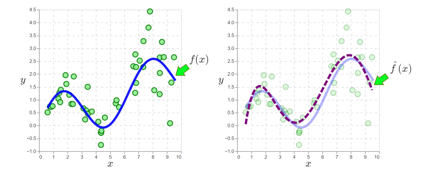 On the left, we have data and the true function \(f(x)\) that generated it. On the right, the data is smoothed to approximate \(f(x)\).
On the left, the \((x, y)\) points are the observed data. The smooth curve is the ‘true’ function we can’t observe, but we assume it generates the data, something like \(y = f(x) + \epsilon\), where \(f(\cdot)\) is the function and \(\epsilon\) is random noise. More explicitly, the data generating process is:
1) An \(x\) is sampled from some unknown distribution.
2) \(x\) is plugged into \(f(\cdot)\) and corrupted with noise: \(y = f(x) + \epsilon\).
This is what we assume gives us the data on the left.
SL moves us to the plot on the right, where the data has been smoothed into \(\hat{f}(\cdot)\), something approximating the true \(f(\cdot)\). With \(\hat{f}(\cdot)\), we can predict \(y\) for any \(x\)4. That’s the goal of SL.
To generalize from SL to CB, we now imagine there are two true unknown functions, one for each of two actions:
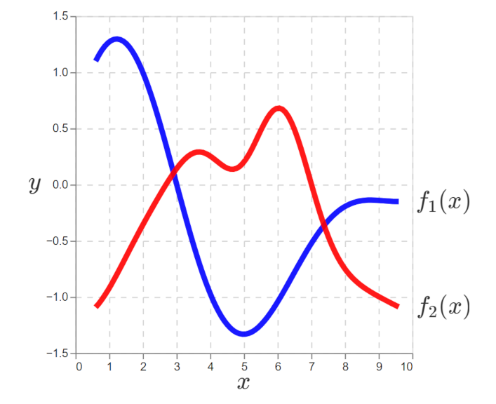 We assume there are two data generating functions, one for each action.
What remains is to specify how actions are selected according to \(x\), which we will now call the context. This is done with a policy, a function \(\pi(\cdot)\) which selects the action \(a\) in a given context.
\[\pi(x) = a\]Now we can write the assumed CB data generating process as a translation of SL:
1) A context \(x\) is sampled.
2) An action is chosen in the context: \(\pi(x) = a\)
3) A reward5 \(y_a\) is generated by the chosen function: \(y_a = f_a(x) + \epsilon\).
I write it this way to make the close connection of SL and CB obvious. They heavily overlap. For instance, if the policy always selected one action, CB would reduce to SL, where we would learn the reward of one action.
From this perspective, the goal is to maximize the reward. That is, averaged over many sampled \(x\)’s, we want a \(\pi(x)\) that produces large positive \(y\)’s.
The Policy Problem
Unfortunately, introducing the policy seriously complicates our job.
To see this, remember our goal is to learn high-reward policies. That means for any \(x\), we should select the max of \(f_1(x)\) and \(f_2(x)\), which means we need approximations \(\hat{f}_1(x)\) and \(\hat{f}_2(x)\), like what SL would provide. To do that, we need data. By the CB process, there must be some policy operating that produced that data.
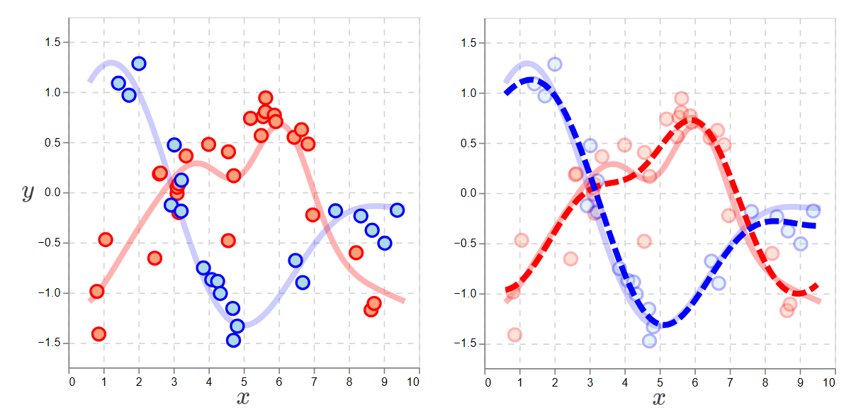
The problem is policies can hide the true functions. Below is a policy that does this. Each data point is colored according to the action selected.
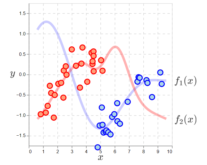 Observations of the two action functions according to a policy that is very likely to select the red action if \(x < 5\).
Choosing an action is to sample an observation from one of the functions.
If the action is fully determined by \(x\), then we never observe one of the functions at every location. This is a blindness.
In the plot, we have no observations of the blue function on the left and no observations of the red function on the right. If we apply SL to these datasets, we see high errors in the unobserved regions:
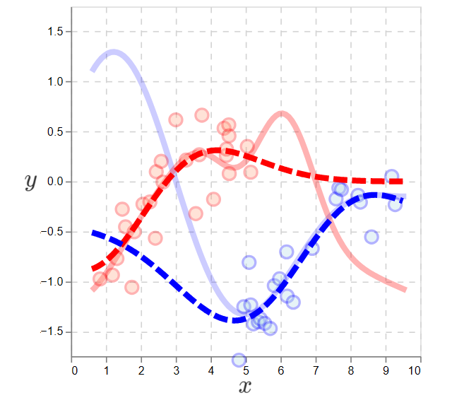 Supervised learning applied to a non-exploratory policy. The dotted lines are the learned functions. On the left, the blue learned function is a poor approximation. Similarly on right, the red is a poor approximation.
To address this, we want policies which do random exploration. That is, for any \(x\), there’s a nonzero probability of selecting any action.
Practically, we need a policy that gathers enough cross-action data to determine which is likely the max action.
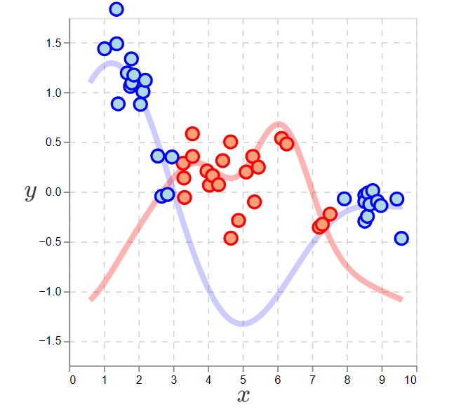
Here is what happens if the policy ignores \(x\) and picks the action by flipping a coin.
 With an exploratory policy, one that selects actions at random, supervised learning can accurately learn the functions of both actions.
With the functions learned, we can set the policy to select the max action:
 Data generated by the optimal policy, the policy that maximizes \(y\)’s.
This shows that by approximately learning \(f_1(\cdot)\) and \(f_2(\cdot)\) via random exploration, we can determine a policy that maximizes expected reward in all contexts. That is, this is nearly the best policy for generating large, positive \(y\)’s.
On Vs Off Policy
By anchoring to SL, where function learning is done with a fixed batch of data, I’ve explained the off-policy version of CB. That is, data is collected under one policy and used to develop another that achieves higher reward. Without getting into the details, off-policy learning, especially when the data isn’t collected under an exploration-oriented policy, is quite hard. It should be avoided if it can be.
So, I’ll switch our presentation to on-policy learning. That is, there’s a single algorithm that both generates the data by choosing actions and is designed to maximize expected reward.
Explore-Exploit
But this raises an issue. As we saw, random exploration is needed to estimate the functions used to construct the optimal policy. However, random exploration is costly in that it foregoes reward; flipping a coin is to select the lesser action half the time. Notice how the optimal policy above does no exploration; it always selects one and only one action depending on the context.
Balancing the learnings produced with random exploration with the reward of exploiting what is known so far is the exploration-exploitation trade-off, something notoriously difficult to management.
Well Optimized Tools
Fortunately, there are strong, well researched opensource algorithms. In a future post, I’ll discuss my favorite tool for apply contextual bandits: Vowpal Wabbit (‘VW’).
If you’re impatient, I’ll recommend two papers for the meantime:
-
A Contextual Bandit Bake-off: Reviewing this paper is what inspired my CB-as-SL perspective, but its utility is well beyond that. I believe it’s essential for understanding VW. The paper turns SL problems into CB problems and compares CB algorithms on these tasks. In doing so, the authors define the CB problem generally, show how SL can be used as a sub-routine, explain many of the VW-implemented CB algorithms, demonstrate their capabilities and offer useful advice for practitioners.
-
Making Contextual Decisions with Low Technical Debt: It should be emphasized that, from an engineering perspective, CB is riskier than SL. CB involves deploying an algorithm that learns on its own as it interacts with the real world. This is a harder thing to evaluate and test than something like a logistic regression model with frozen coefficients. Further, CB agents involve information that isn’t typically stored in the same locations. Things like a decision and its probability need to be as primary as the \(y\) variable. So CB presents unique engineering challenges. In the discussion of their solution (the Decision Service), this paper, authored by the VW people, discusses those challenges and how they should be handled.
You can also check out the VW Wiki, but as you’ll see, you need to read the surrounding research to understand what VW is doing. That’s why I’d start with these two papers.
References
-
A. Agarwal, et al. Making Contextual Decisions with Low Technical Debt. arXiv:1606.03966v2. May 9, 2017.
-
P. Henderson, et al. Integrating Reward Maximization and Population Estimation: Sequential Decision-Making for Internal Revenue Service Audit Selection. arXiv:2204.11910v3. Jan 24, 2023.
-
D. Bouneffouf, I. Rish. A Survey on Practical Applications of Multi-Armed and Contextual Bandits. arXiv:1904.10040v1. April 2, 2019
-
L. Li, W. Chu, J. Langford, R. Schapire. A Contextual-Bandit Approach to Personalized News Article Recommendation. arXiv:1003.0146v2. March 1. 2012
-
A. Bietti, A. Agarwal and J. Langford. A Contextual Bandit Bake-off. arXiv:1802.04064v5. 2021
Something to Add?
If you see an error, egregious omission, something confusing or something worth adding, please email dj@truetheta.io with your suggestion. If it’s substantive, you’ll be credited. Thank you in advance!
Footnotes
-
I say ‘arguably’ because it depends on how reinforcement learning is defined. If it’s defined as involving an agent that learns, interacts and accrues reward in the real world, contextual bandits are surely a top contender. If it’s defined as any reward optimization over a simulation, the argument becomes weaker. In such a case, some massive logistical network optimizations would also count as applied RL, and those could certainly dethrone contextual bandits. ↩
-
The link points to code that eHarmony uses to deploy Vowpal Wabbit, Microsoft’s opensource online-learning and contextual bandit tool. ↩
-
The context can also include information relating each action to the user. ↩
-
(Excuse me if this is obvious) SL normally deals with vector inputs \(\mathbf{x}\) and real-valued or categorical \(y\)’s. ↩
-
It should be noted that \(r\) is the typical reward notation, but I’m using \(y\) to connect CB and SL. ↩