TrueSkill Part 1: The Algorithm

Who is the greatest boxer of all time? Who is the ‘GOAT?’ Is it Muhammad Ali? Mike Tyson? Someone else?

Because they never fought each other, you might say it can’t be known. Indeed, it can’t be known, but it can be estimated.

The absence of a prime Tyson vs prime Ali match does not mean we have no evidence. Something can be inferred from Tyson’s win over Larry Holmes and Larry Holmes’ win over Ali. Additional evidence comes from a chain of two fighters, one who fought Tyson, one who fought Ali and who fought each other. Still more evidence comes from a chain of three fighters, and so on. Collectively, across all chains, there’s substantial evidence to predict the outcome of the Tyson vs Ali fight.

An immediate critique is that Ali fought Holmes at the end of his career and Tyson fought him near his prime. This effect can be handled as well, with an assumption that skill evolves incrementally over time and with experience.

Introduced in Herbrich et al. (2007), the TrueSkill algorithm captures these effects beautifully. With some extensions, Microsoft deploys it at scale to matchmake many millions of gamers annually. Beyond its applied utility, it is an exceptional victory for Bayesian methods, where simple assumptions and probabilistic reasoning produce accurate estimates of counterfactual matchups.

Further, the algorithm is game agnostic. All that is needed is when-and-who data on matches. As such, it can be applied to boxing, tennis, chess, MMA, and others. In fact, it can be applied to arbitrarily team multiplayer games, like Halo.

The Elo Rating System

To motivate, let’s consider the issue with counting metrics to evaluate skill. If you were to evaluate a chess player’s skill, which metric would you use? Win Rate?

That creates a problem. Win rate doesn’t account for the strength of the opponent. A win rate of 20% against exclusively Magnus Carlsen, arguably the GOAT, is much more impressive than a 90% win rate against an amateur.

This is why the Elo rating system is used for chess and many other two player games.

The idea is to assign skill values to players and to model the probability of a win as the difference of their skills. If player 1 has skill \(s_1\) and player 2 has skill \(s_2\), the probability player 1 wins is model as¹:

\[\Phi\Big(\frac{s_1 - s_2}{\sqrt{2}\beta}\Big)\]

where \(\Phi(\cdot)\) is the cumulative density of a standard normal distribution. It looks like:

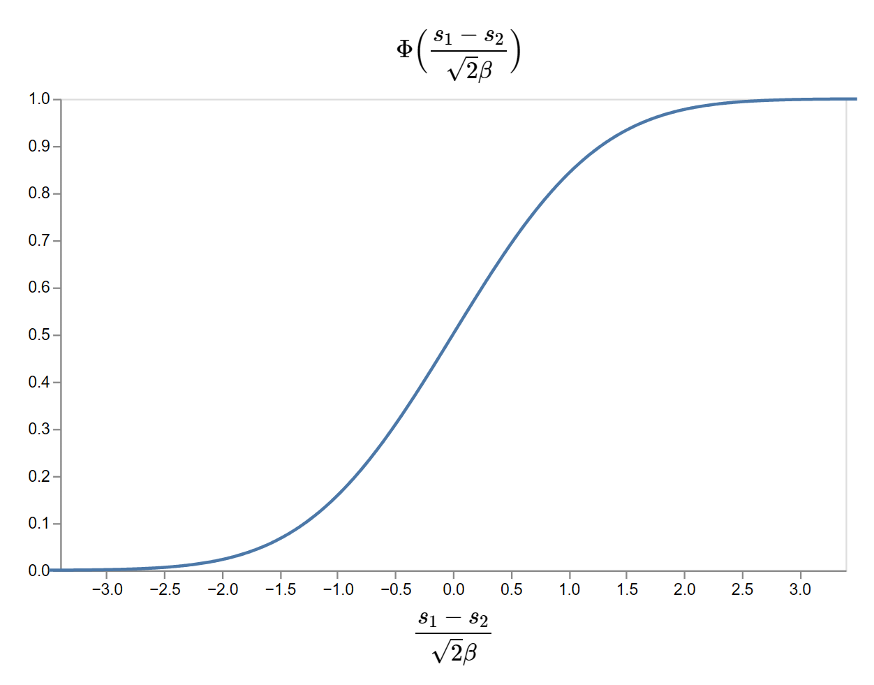The cumulative density function of the standard normal distribution. It is chosen for its S-shape, nothing more.

The effect is that if player 1 is much more skilled than player 2, \(s_1 - s_2\) is large and positive and the probability of plyer 1 winning is close to one. Similarly, it’s close to zero when player 2 is much more skilled than player 1. \(\beta\) is a tunable parameter to set what counts as ‘large’.

This becomes useful when we have \(N\) players who have played each other many times. Per maximum likelihood estimation, we can estimate \(s_1, s_2, \cdots, s_N\) by applying the win probability to all observed games and finding those that make the observations most likely.

The key is that skills are estimated jointly. They are inferred simultaneously, from observed match outcomes to skill differences to skill values. This means all skills are determined in relation to each other, such that skill differences explain the data maximally well.

Admittedly, I’ve oversimplified things. In practice, skills evolve over time and the optimization can be converted into convenient update rules to be applied after each match. Regardless, this online procedure does not contradict the skills’ relative definition.

Problems with Elo

In 2005, Microsoft Research considered Elo when looking to improve their matchmaking for XBox Live and Halo specifically.

Elo wasn’t the answer for a few reasons:

• There is no measure of uncertainty. Surely, there should be something separating the skill of a player who has played once and another who has played 100+ times.
• It only applies to two player games. Complicating things, Halo normally involves more than two players.
• There are no teams. Halo could involve free-for-all matches or team-based play.

TrueSkill: What It Does

In 2006, TrueSkill was invented in response, and it has since stood the test of time.

To understand it, we’ll begin with TrueSkill’s assumptions. It assumes the data is produced by a certain data generating process or simulation. Rather than describing it precisely and in its full generality, I’ll illustrate the essentials.

Suppose there are \(N\) players playing over \(M\) matches. In fact, with loss of generality, we’re treating the match index like a time index, as though there were one match per timestep, involving all players. Further, each match could be a free-for-all, or with two-player teams, or three-player teams. This is also a loss of generality, since TrueSkill works with arbitrary teams.

Next, we assume players skill evolve as random gaussian walks over the matches. With three players, that looks like:

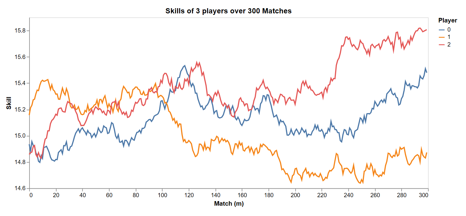The match index \(m\) acts like a time index, where we assume there is one match per day involving all players. In this case, skills of three players evolve like a gaussian random walk.

This can be expressed as \(s_{i, m+1} \sim \mathcal{N}(s_{i, m}, \gamma^2)\), where \(s_{i, m}\) is player \(i\)’s skill at match \(m\) and \(\gamma\) is a parameter of the simulation, giving the standard deviation of skill change with each match.

The match outcome is simulated as follows. \(p_{i, m}\) is player \(i\)’s performance on match \(m\) and is normally distributed around their skill. That is, \(p_{i, m} \sim \mathcal{N}(s_{i, m}, \beta^2)\). The standard deviation of performance, \(\beta\), indicates the game’s noisiness. Poker, with its element of chance, has a higher \(\beta\) than chess. For two players and a game without draws, their performances are normally distributed about their skills and the winner, denoted with a green dot, has the higher performance.

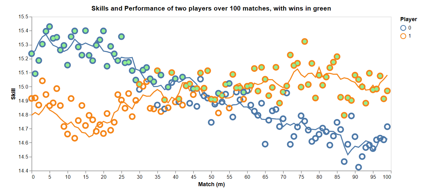Performances, indicated as circles, are normally distributed, centered on player skill. In this two player game without draws, the player with the higher performance wins, indicated with a green dot.

In the style of Elo, the probability of a win for player 1 on match \(m\) is:

\[\Phi\Big(\frac{s_{1, m} - s_{1, m}}{\sqrt{2}\beta}\Big)\]

However, unlike Elo, TrueSkill can handle teams. To do this, it assumes the performance of the team is the sum of its players’ performances. If there were \(N=6\) players with three teams of two, then:

\[\begin{align} t_{1, m} &= p_{1, m} + p_{2, m}\\ t_{2, m} &= p_{3, m} + p_{4, m}\\ t_{3, m} &= p_{5, m} + p_{6, m} \end{align}\]

In this case, the team with the highest performance wins. Similar to the two player case, the probability that team 1 ranks above team 2 in match \(m\) is:

\[\Phi\Big(\frac{(s_{1, m} + s_{2, m}) - (s_{3, m} + s_{4, m})}{\sqrt{2}\beta}\Big)\]

It should be noted that in multi-team matches, the outcome is not binary; it is a ranking of teams. In a three team match, a match outcome might be \(2, 3, 1\), showing team \(2\) came in first and team \(1\) came in last. These rankings and which players are on which teams constitution the observations; we know their values when applying TrueSkill. Picture that like this:

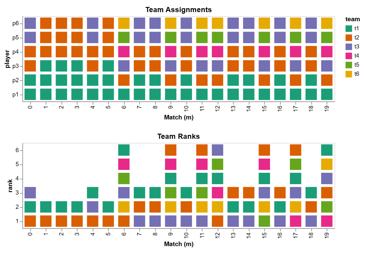The top plot shows which team each player is on for every match. The bottom plot shows the team rankings for every match.

Using only the data shown here, TrueSkill infers players skills and provides uncertainties, quantifying the inference quality.

Seeing this inference is what is enabled by our simulation. We can feed TrueSkill the generated observations, pull out skill estimates and their uncertainties, and compare them to the simulated skills. For one player, we get:

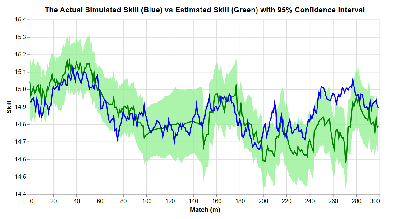For a player, TrueSkill infers their skill from the match outcomes.

This gives the spirit of TrueSkill, but to show this, a cheat was necessary. Methods like this run into the problem of identifiability; skills cannot be uniquely inferred from observations. One reason is that the probability of a match outcome depends only on skill differences, and there is a whole range of skill pairs with a given skill difference². So to create this satisfying recovering-of-the-truth, I allowed TrueSkill to know the actual skill of one player. This anchored the other estimates.

In applied cases, identifiability is not an issue for TrueSkill. It is anchored to match outcome probabilities, and those are the essential ingredients to matchmaking and the primary counterfactual question. In other words, we only care about skill differences and those can be uniquely determined.

TrueSkill: How It Works

The math is sophisticated and detailed, so I will go just deep enough to capture the basics. We will follow the presentation of Herbrich et al. (2007), and explain the computation of a single match, ignoring the random walk of skills over matches. If \(\mathbf{s}\) is a vector of player skills for a match, the goal is to compute its posterior distribution given the observation. That is, we want:

\[p(\mathbf{s} \vert \mathbf{r}, A)\]

where \(A\) tells us which players are on which teams and \(\mathbf{r}\) is the team rankings. Ultimately, we won’t be concerned with the full joint distribution over \(\mathbf{s}\). Rather, we will model each \(s_i\) with a normal distribution, where its mean and variance are the skill estimate and uncertainty we seek. This skill distribution for player \(i\) will be conditional on \(\mathbf{r}\) and \(A\), and on the estimates of the other players.

The example considered has player 1 on team 1, players 2 and 3 on team 2 and player 4 on team 3. The rankings are \((1, 2, 2)\); team 1 came in first and teams 2 and 3 tied for second. We have thus far avoided ties, but these are supported in TrueSkill. Teams tie when their performance is within some small difference \(\epsilon\). In this case, \(\vert t_2 - t_3 \vert < \epsilon\).

To compute the posterior over skills, we must integrate out all possible performances, for both teams and players. Written out explicitly, \(p(\mathbf{s} \vert \mathbf{r}, A)\) is equal to the follow integral:

\[\small \int_\infty^\infty \int_\infty^\infty \int_\infty^\infty \int_\infty^\infty \int_\infty^\infty \int_\infty^\infty \int_\infty^\infty p(\mathbf{s}, p_1, p_2, p_3, p_4, t_1, t_2, t_3 \vert \mathbf{r}, A)dp_1dp_2dp_3dp_4dt_1dt_2dt_3\]

In this generic form, this is not an easy calculation, even for a single match. However, we can exploit structure in the TrueSkill assumptions for efficiency.

To see this, we start with computing the integrand, more compactly expressed as \(p(\mathbf{s}, \mathbf{p}, \mathbf{t} \vert \mathbf{r}, A)\). This computation is represented with Figure 1 from Herbrich et al. (2007), copied here:

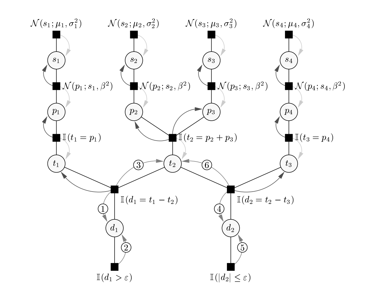This is a factor graph representing the computation of \(p(\mathbf{s}, \mathbf{p}, \mathbf{t} \vert \mathbf{r}, A)\) under the TrueSkill data generation assumptions.

This is a factor graph representation of \(p(\mathbf{s}, \mathbf{p}, \mathbf{t} \vert \mathbf{r}, A)\), where \(\mathbf{r}=(1,2,2)\) and \(A\) represents the team participations, as described. To be clear, \(\mathbf{r}\) and \(A\) dictate the shape of the graph. Just like \(p(\mathbf{s}, \mathbf{p}, \mathbf{t} \vert \mathbf{r}, A)\), think of this graph as something that receives values of \(\mathbf{s}, \mathbf{p}, \mathbf{t}\) and gives back a number. Though it is more than that, as we’ll see.

Computing \(p(\mathbf{s}, \mathbf{p}, \mathbf{t} \vert \mathbf{r}, A)\) involves a product of factors, which are functions of variables. To understand this, we explain the factor graph.

A factor graph has two types of nodes. Large circles (so not including the small numbered circles) represent random variables. The first row of circle nodes labeled \(s_1, \cdots, s_4\) are the player skills as of this match. The second row, labeled \(p_1, \cdots, p_4\) are player performances. The third row, labeled, \(t_1, t_2, t_3\) are team performances. The last row gives rank-consecutive team performance differences. That is, \(d_1 = t_1 - t_2\) and \(d_2 = t_2 - t_3\). As will be discussed next, these variables are introduced to assert the given \(\mathbf{p}\) and \(\mathbf{t}\) are consistent with \(\mathbf{r} = (1,2,2)\).

Black square nodes represent factors, functions of those random variables that connect with them. So the top row of black squares are four functions of \(s_1, s_2, s_3, s_4\) respectively. In fact, they are normal densities under \(\mu_i\) and \(\sigma_i\), representing their prior distributions (or distributions conditional on previous matches). The next row of black squares represent the densities of performances given skills and \(\beta\). The third row of black squares are indicator functions checking whether the team performances in fact sum to the player performances. This is to zero-out combinations of \(\mathbf{p}\) and \(\mathbf{t}\) that don’t match that definition. The second to last row and last row define \(d_1\) and \(d_2\) and indicate whether they are such to produce the \(\mathbf{r}=(1,2,2)\) ranking.

The factor graph instructs a faster computation than the generic six-nested integral. This is because each factor only concerns a small subset of variables, those connected to it. Put simply, given \(\mathbf{s}, \mathbf{p}, \mathbf{t}\), we could compute products of factors, starting from the top black squares and cascading downwards, producing a number equal to \(p(\mathbf{s}, \mathbf{p}, \mathbf{t} \vert \mathbf{r}, A)\). If the given \(\mathbf{s}\), \(\mathbf{p}\) and \(\mathbf{t}\) were inconsistent with \(\mathbf{r}\) and \(A\), the result is zero. That is the purpose of the indicator functions seen in the graph.

What remains is to integrate out \(\mathbf{p}\) and \(\mathbf{t}\) from \(p(\mathbf{s}, \mathbf{p}, \mathbf{t} \vert \mathbf{r}, A)\). This is done with Expectation Propagation (EP), a message passing algorithm from the category of variational inference methods. This is an extensive topic, so I will be brief. Essentially, the integration can be approximated with an iterative but fast computation that proceeds down and up the graph, as indicated with light-to-dark curved arrows. The messages flowing through the graph all take the form of univariate normal distributions, even for the non-gaussian portions of the graph near the indicator functions. Gaussians are chosen because they make products and integrals easy.

For some intuition on variational methods, see Part 3 of my series on Probabilistic Graphical Models. For a more complete explanation, see Herbrich et al. (2007) or section 22.5 of Murphy (2012).

The point is we can approximate the integral with an efficient computation over this graph, made possible by the TrueSkill assumptions and the EP algorithm. Further, it is simply combined with the random walk of skills over matches; the same up-down routine can be used to update skill estimates with each new match.

Doing so provides a univariate distribution over each player \(i\)’s skill \(s_i\), with mean \(\hat{\mu}_i\) and standard deviation \(\hat{\sigma}_i\). These values represent not only who a player has beaten, but who the beaten player has beaten, and so on, for all chains of matches. Naturally, these skills are used to rank players. For XBox Live, players were ranked according to a conservative skill estimate of \(\hat{\mu}_i - 3\hat{\sigma}_i\).

Most importantly, given any two players, including those who have never played each other, we can accurately estimate the probability of a win or loss.

TrueSkill Performance

In Herbrich et al. (2007), there are several quantifications and plots demonstrating TrueSkill’s efficacy. One that I found especially convincing is copied here:

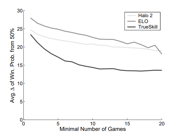An optimal matchmaking system will ensure one-on-one games have close to a 50% probability of player 1 winning. However, in real applications, it takes some games for the system to determine skill levels, to make those 50-50 matches. For each skill measure, this skill plot shows the difference from 50% of the empirical win-rate. A value of 0 is optimal. This plot shows that TrueSkill is closer to 0 and approaches it more quickly then Elo or the Halo 2 ranking system.

TrueSkill Variants

Since TrueSkill’s publishing, there have been several notable extensions:

• TrueSkill Through Time (Dangauthier (2008)): An interesting limitation of vanilla TrueSkill is that skill estimates depend only on past matches. However, suppose a player defeated someone who later became the champion. In retrospect, the estimate of the player who beat the champion should be revised upward. This is the difference between vanilla TrueSkill, performing filtering, and TrueSkill Through Time, performing smoothing. Smoothing is the better option for retroactively determining the GOAT.

  Another element is that vanilla TrueSkill assumptions skills only change with matches. TrueSkill Through Time assumes skills evolve over time. This is more realistic, since it is likely that matches occur outside of the data or skills change due other time related factors, like age.

• TrueSkill 2 (Minka (2018)): Vanilla TrueSkill only operates on wins, losses and draws, but in most games, there’s other useful information. TrueSkill 2 is an extension to factor in, among other things, players quitting matches, death/kill ratios, and correlations across match types.

• Multidimensional Skill (Chen (2016)): While not a TrueSkill variant, it is worth mentioning. An assumption of TrueSkill is that a skill is a single number. However, players and their styles might not be so simply modeled. We could have an arrangement like rock-paper-scissors, where player 1 has an advantage of player 2, who has an advantage of player 3, who has an advantage of player 1. This presence intransitivity; observing player 1 beating player 2 many times and player 2 beating player 3 many times may not be enough to confidently say player 1 will beat player 3. It should noted that this is an exotic effect to capture, and most systems consider univariate skills.

The Details

For those interested in the details of the above analysis, see this notebook. It relies on the TrueSkill implementation by Heungsub Lee.

Part Two

We have briefly toured the ingenious True Skill algorithm, but we’ve yet to see it applied to real data. In an upcoming post, we will apply it to boxing, tennis and warcraft 3, a classic real time strategy game.

---

References

1. R. Herbrich, T. Minka, T. Graepel. TrueSkill(TM): A Bayesian Skill Rating System Advances in Neural Information Processing Systems. January 2007

2. P. Dangauthier, R. Herbrich, T. Minka, T. Graepel. TrueSkill Through Time: Revisiting the History of Chess In Advances in Neural Information Processing Systems. MIT Press, January 2008

3. T. Minka, R. Cleven, Y. Zaykov. True Skill 2: An improved Bayesian skill rating system. Microsoft. March 2018

4. S. Chen, T. Joachims. Modeling Intransitivity in Matchup and Comparison Data Association for Computing Machinery. 2016

5. K. Murphy. Machine Learning: A Probabilistic Perspective. MIT Press. 2012.

---

Footnotes

1. In practice, the ELO system is slightly different. Beta is used to scale skills to be in the range of a few thousand. Also, the logistic function, rather than the normal CDF, is used for compute purposes. ↩

2. Some of this is relieved with a prior distribution over skills, but that only mitigates the issue. For instance, if one player always beats another player, then there is a huge range of plausible skill pairs. They need only have at least some large skill difference. A prior will bias this difference to be smaller, but the truth of the matter may be a much larger difference. ↩